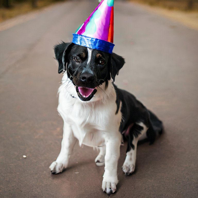
Diffusion models are now the go-to models for generating images. As diffusion models allow us to condition image generation with prompts, we can generate images of our choice. Among these text-conditioned diffusion models, Stable Diffusion is the most famous because of its open-source nature.
In this article, we will break down the Stable Diffusion model into the individual components that make it up. Also, we will understand how Stable Diffusion works.
Getting familiar with the working of Stable Diffusion will allow us to understand the process of its training and inference as well.
After understanding the conceptual part of Stable Diffusion, we will cover the different versions and variations of it.
- What is Stable Diffusion?
- Different Components of the Stable Diffusion Model
- Training Stable Diffusion
- Stable Diffusion Inference – Generating Images from Noise and Prompt
- Different Versions of Stable Diffusion
- Summary
What is Stable Diffusion?
Originating from the Latent Diffusion Model (LDM), which was the original text-to-image model, Stable Diffusion is an extension. This means that Stable Diffusion is also a text-to-image model.
The original open source code by CompVis and RunwayML is based on the paper – “High-Resolution Image Synthesis with Latent Diffusion Models” by Rombach et al.
Feeling perplexed about diffusion models and their mechanisms? Don’t fret, as we have you covered. Our article on Denoising Diffusion Probabilistic Models delves into them comprehensively. Moreover, you will also have the opportunity to build a basic diffusion model from scratch using PyTorch.
As you may have guessed by now, Stable Diffusion is not the only diffusion model that generates images.
Prior to Stable Diffusion there was DALL-E 2 by OpenAI. Following that, Google released Imagen. Both of these are text-to-image diffusion models.
This raises a pertinent question – “How is Stable Diffusion different from other diffusion models that generate images from prompts?”
Let’s answer that question in the next section.
How is Stable Diffusion Different from Other Diffusion-Based Image Generation Models?
Stable Diffusion works on the latent space of images rather than on the pixel space of images.

Other generative diffusion models like DALL-E 2 and Imagen work on the pixel space of images. This makes them slower and, in the process, consumes more memory.
An Autoencoder model helps create this latent space which also works as the noise predictor in the model. If you have gone through the previous DDPM post, then you already know that a noise predictor model is an indispensable part of an LDM (Latent Diffusion Model).
At this point, a few additional questions come to mind.
- Is UNet one of the components/models in the Stable Diffusion model?
- Are there other components in the model? If so, what are they?
Different Components of the Stable Diffusion Model
We can break down the Stable Diffusion model into three primary components:
- A pre-trained text encoder
- An UNet noise predictor
- An Variational autoencoder-decoder model. The decoder also contains an Upsampler network to generate the final high-resolution image.
But all the components are involved during both training and inference. During training, the encoder, UNet, and pre-trained text encoder are used. While during the inference, the pre-trained text encoder, the UNet, and the decoder are involved.
Speaking at a very high level, a pre-trained text encoder converts the text prompt into embeddings.
The UNet model acts on the latent space information as the noise predictor.
The autoencoder-decoder has two tasks. The encoder generates the latent space information from the original image pixels and the decoder predicts the image from the text-conditioned latent space.
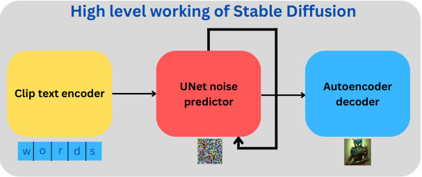
We will go through the working of each component but not in individual sections. Instead, we will understand their workings from the perspective of training Stable Diffusion and carrying out inference.
Training Stable Diffusion
Training a Stable Diffusion model involves three stages (keeping aside the backpropagation and all the mathematical stuff):
- Create the token embeddings from the prompt. From a training perspective, we will call the text prompt the caption.
- Condition the UNet with the embeddings. The latent space is generated using the encoder part of the autoencoder model. This is called text conditioned latent space.
- The UNet entirely works on the latent space.
- From the above step, the UNet predicts the noise added to the latent space and tries to denoise it.
Text Encoder
Generally, in all diffusion models, the text encoder is a large pretrained transformer language model.
Stable Diffusion uses the pre-trained text encoder part of CLIP for text encoding. It takes the caption as input and outputs a 77×768 dimensional token embedding.
Why 77 though?
Out of the 77 tokens, 75 are text tokens from the caption, 1 for the start token, and 1 other for the end token.
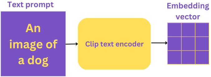
Other pre-trained language transformers models like T5 and BERT may also be used. But Stable Diffusion uses CLIP.
Google’s Imagen uses a T5-XXL transformer model for text encoding.
The UNet Noise Predictor
Before the UNet, the encoder part of the autoencoder-decoder model converts the input image into its latent representation.
Now, it’s important to remember that the UNet acts exclusively on the latent space and does not deal with the original image pixels at all. It is, of course conditioned by the text caption. The process of adding the caption information to the latent space is called text conditioning.
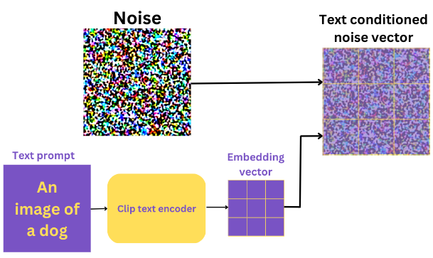
Not just text conditioning, the latent information also goes through a noise addition step, as discussed above.
From all the above information, the UNet tries to predict the noise added to the image.
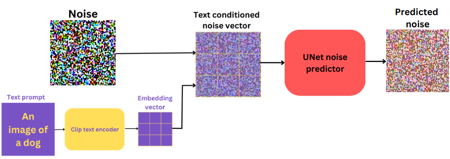
But that’s not all. The UNet architecture is more complex than this. It contains Residual layers for skip connections and Attention layers for merging the text information into the image’s latent space.
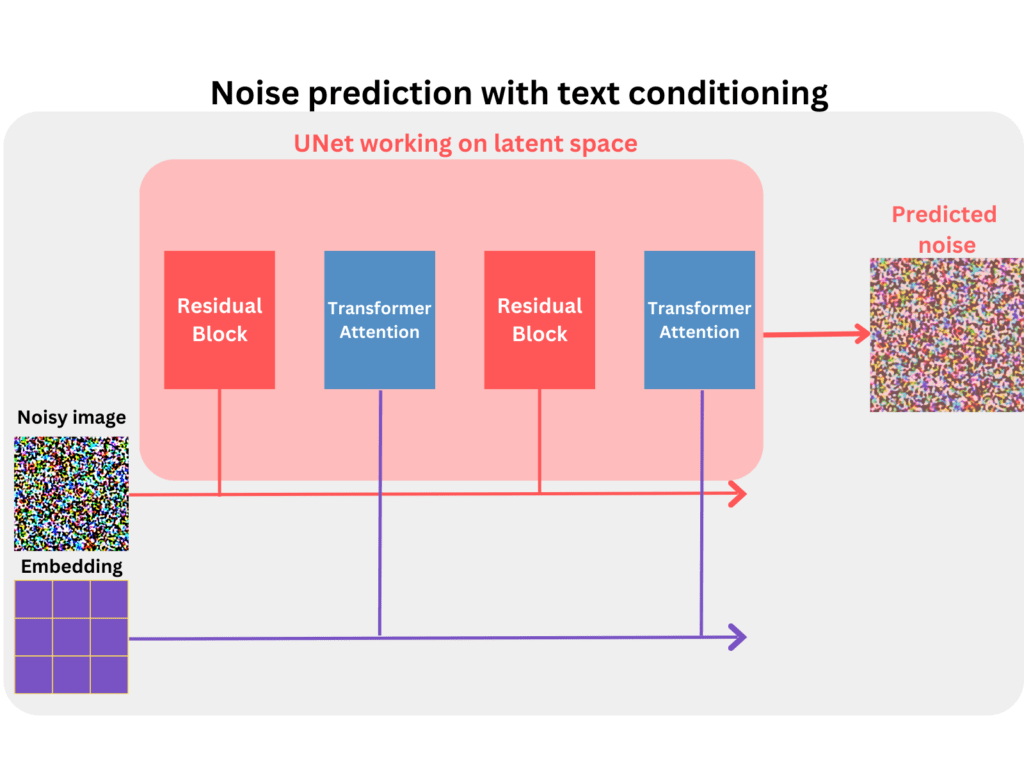
After the merging step, the Residual blocks can utilize the embedded information in the denoising step.
The UNet outputs a 64×64 (spatial) dimensional tensor.
We discussed how the latent had been conditioned on the text caption. But we can also condition the same latent space with semantic maps or other images. More on this in future posts.
The Autoencoder-Decoder Model
As previously discussed, the encoder part of the autoencoder model creates the latent space from the original image.
Finally, the decoder part of the model is responsible for generating the final image.

The decoder acts on a 4x64x64 dimensional vector and generates a 3x512x512 image. The original Stable Diffusion model (till version 2.0) generates a 512×512 dimensional image by default.
The Entire Process of Training Stable Diffusion
As shown in the original LDM paper, the entire process can be summarized in the following image.
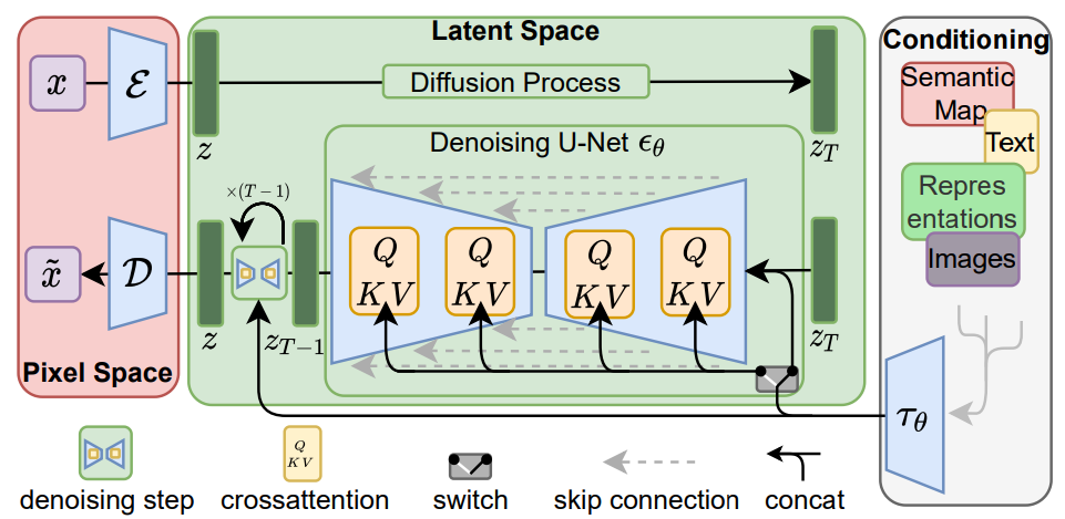
Figure 9. Stable-diffusion-training-process-ldm-paper.png
You can see how first the encoder encodes the image into a latent space (top part right red block). And notice how we can condition the latent space with either text, semantic map, or even images.
The QKV blocks represent the cross-attention from the Transformer model. The big green block shows the working of the UNet on the latent space to predict the noise.
Stable Diffusion Inference – Generating Images from Noise and Prompt
Once we have a trained Stable Diffusion mode, generating images goes through a slightly different process than training.
During inference, we don’t have an image with us initially. Instead, we have to generate one using a text prompt. Also, we do not need the encoder part of the autoencoder-decoder network. This boils down the inference components to the following:
- The pretrained text encoder.
- The UNet noise predictor.
- And the decoder part of the autoencoder-decoder network.
The Process of Generating Images from Prompts
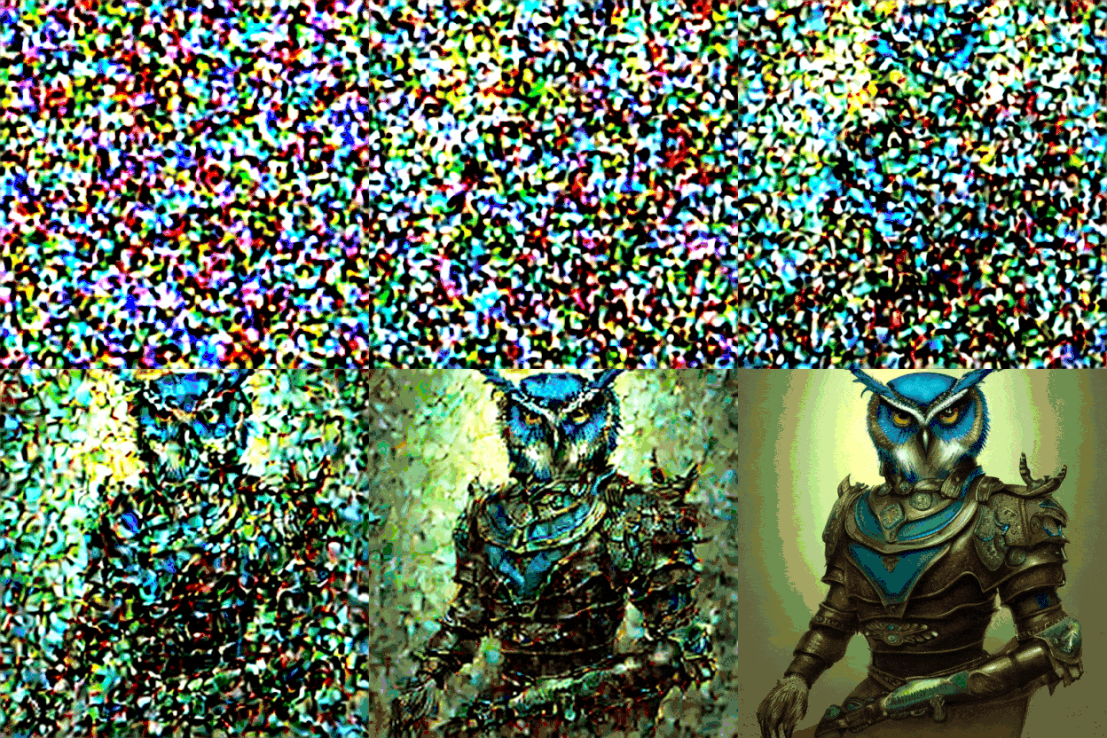
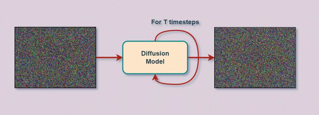
Instead of adding noise to an image, we start directly with pure Gaussian noise. The Stable Diffusion model then iteratively denoises it to generate the final image. We can control the number of denoising steps, which is called sampling steps.
If it is a pure diffusion model (not conditioned on text prompt), then the process will be similar to the following:
But here, we have a text prompt, and the noise needs to be conditioned on the text prompts. So, the process looks like this:
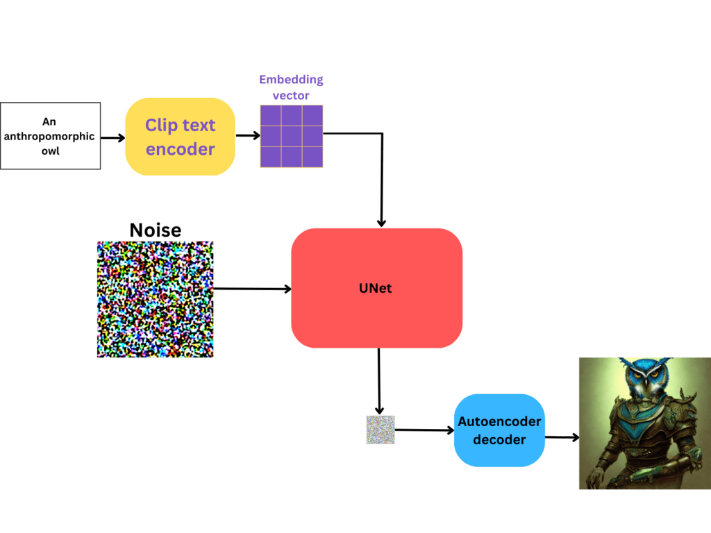
Apart from the input image and the encoder (which we don’t need anymore), every other component remains the same.
But, we spoke about sampling steps just above. How does that look in this entire process?
This can be better explained by expanding the UNet and showing the denoising process.
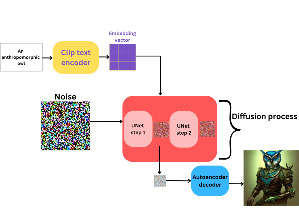
We can call the above process the reverse diffusion process, as the model generates images from noise.
Some Practical Considerations
Here are some points to clarify a few concepts about the inference stage:
- The input prompt need not b 75 words long exactly. We can also provide shorter and longer prompts as well.
- During inference, the UNet still generates an image with a 64×64 spatial dimension.
- The decoder part of the autoencoder is both an upsampler and a super-resolution model combined. This generates the final 512×512 image.
- But as of today, from a completely practical perspective, we can generate images of any resolution as long as we can afford the GPU memory.
We have thoroughly discussed the training and inference of Stable Diffusion, thus marking the end of a long theoretical journey. Moving forward to the next section, we will explore various versions and variations of Stable Diffusion.
Different Versions of Stable Diffusion
Since its release, Stable Diffusion has undergone many revisions and updates.
Stable Diffusion was initially introduced as version 1.4 by CompVis and RunwayML, followed by version 1.5 by RunwayML. The current owner, StabilityAI, maintains the latest iterations, Stable Diffusion 2.0 and 2.1. These are the official versions of Stable Diffusion. In addition, there exist numerous finely tuned Stable Diffusion models that can produce images in specific art styles. We will delve into them further in the upcoming section.
Variations of Stable Diffusion
Here, we will discuss some of the more famous variations of Stable Diffusion among the many that are out there.
All of these models are obtained by fine-tuning one of the base Stable Diffusion versions.
Do you also want to fine-tune Stable diffusion on your own images? If yes, then do take a moment to check out our new AI Art Generation course on Kickstarter.
Here you will learn how to fine-tune Stable Diffusion on your own images using two of the most popular methods, DreamBooth and Textual Inversion. After this, you will have the skill to generate your own AI Avatars in any style you want. Additionally, you will also learn how to train a GPT language model for Advanced Prompt Engineering to speed up the process of AI Art Generation, from ideation to execution
You can find all of these models (trained weight files on Hugging Face)
Arcane Diffusion
This variation of Stable Diffusion has been fine-tuned on images from the TV show Arcane.

When giving a prompt to the model, simply adding the words arcane style will generate the image in Arcane art style.
Robo Diffusion
The Robo Diffusion version of Stable Diffusion can generate really cool images of robots.
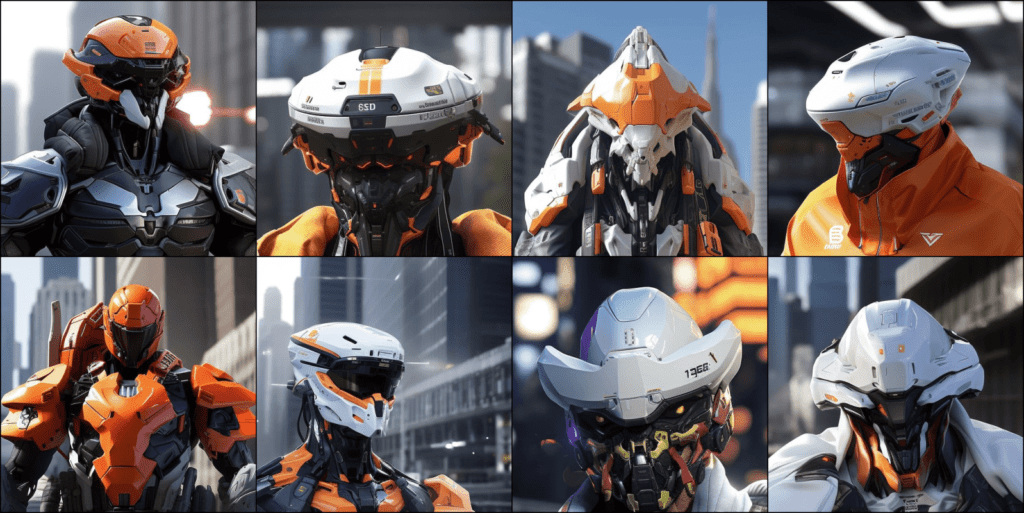
The above images are generated using Robo Diffusion version 2.
Open Journey
The Openjourney model can generate images in the style of Midjourney.
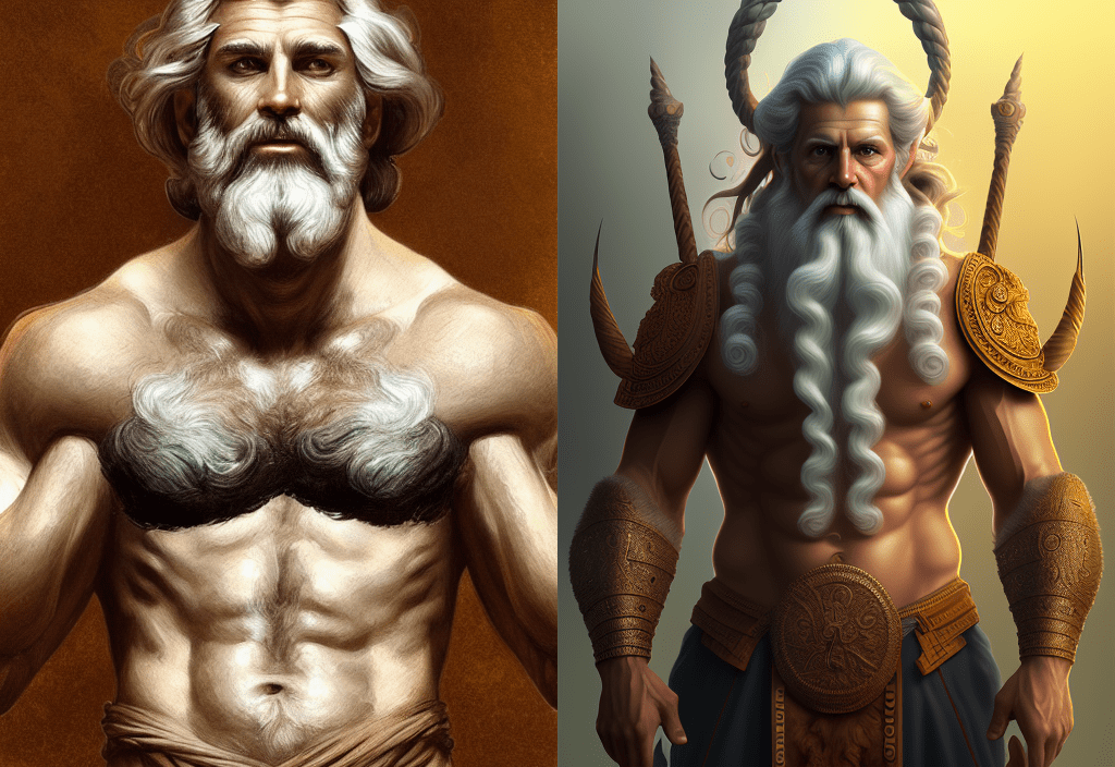
These images are much more artistic and dynamic compared to the base Stable Diffusion model. The Openjourney model has been trained on image outputs from Midjourney.
Mo Di Diffusion
The Mo Di Diffusion model adds Disney art style to any image that we create.
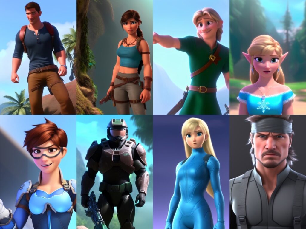
Although not clearly known at the moment, this is a Stable Diffusion 1.5 model which has been fine-tuned on images from an animation studio.
Summary
In this article, we covered the entire architecture of Stable Diffusion. Along with training and inference, we also covered the variations of Stable Diffusion.
As you can interpret from this article, open sourcing models (like Stable Diffusion) lets the AI community expand the scope of usage. Starting from very simple characters to sophisticated ones in different art styles, these models let us explore our creativity. Further, the computation needed to fine-tune these models are decreasing. Almost anyone with a very modest consumer GPU can fine-tune a Stable Diffusion model.
So, what are you going to build with Stable Diffusion? Let us know in the comment section.
References
- Paper: High-Resolution Image Synthesis with Latent Diffusion Models
- High-Resolution Image Synthesis with Latent Diffusion Models

