In today’s blog post you will learn how to train your own fast style transfer network in PyTorch and deploy the model to get live style transfer effect on a web meeting on Zoom/Skype/ Microsoft Teams or Hangouts, all in real-time. This works on Linux, Mac and Windows and the method described here could be extended to demonstrate any kind of computer vision pipeline like object detection or semantic segmentation. Not only is this a good way to learn about computer vision, stylizing your video feed with the logo/flag of your favorite sports team is a great way to enjoy live sports watch parties.
Overview
This blog post is divided into four parts:
- Introduction to style transfer: First we will introduce the basic ideas behind style transfer and explain the modification to the original algorithm which enables real time inference.
- Building style transfer network: We will identify the components needed to build the style transfer network and write them as different modules. Finally we will combine these modules into a pipeline and train the model.
- Creating a virtual camera in Linux/macOS and Windows: We will discuss how to create a virtual camera in all major operating systems, which we can write to.
- Running style transfer in a Zoom meeting: Finally, we will use the model we trained and create an inference pipeline which will write the stylized video data to the virtual camera. This camera can be read by any video calling but we will use Zoom for the demonstration.
A brief background
Around the middle of the last decade, deep learning had already taken the field of computer vision by storm. After Alex Krichevsky’s seminal paper on image classification with Convnets, the field was thrown wide open to build upon their work and apply deep learning to new fields. A few months after Ian Goodfellow introduced the now celebrated idea of generative adversarial networks, which could generate highly realistic-looking images (or so was the promise back then, which has since been realized), Gatys etc. al. showed a completely new application of deep learning by showing how neural networks could be used to apply artistic filters to images so that the resulting images were realistic with artistic styles blended into them.

The general Style Transfer Algorithm
Problem Definition
As shown in the above figure, we start with a pre-trained image classification model, M (such as VGG16), an artistic image, A and a photograph P. Our objective is to find an image X, which has the visual style of artwork A (called style target) and the semantic content of photograph P (called content target).
Insight
The key insight is that the image classification model has already learnt high level representations of the visual information, both content and style, in natural images and we can make use of its learnt representations to guide our search.
Style Representation
The style of A can be represented by so called gram matrices of the hidden layers of the network. Suppose, we pass a single image through the model M and the output of the k-th layer of M is a 1x128x28x28 tensor (in NCHW format). If we flatten this tensor along the width and height dimensions (and ignore batch dimension), we can interpret the resulting 128×784 matrix (call it R) as 128 different representations of the image in a 784 dimensional space. We know that different convolutional channels in a neural network encode different kinds of information, so knowing which ones fire together in an image and which ones don’t can serve as a greatly useful representation of the style of the image. This is mathematically known as cross correlation and it can be calculated as RRT, which will be a 128×128 sized matrix in this case. We call this style representation of A as GA.
Content Representation
The content representation of the image is much more straightforward. The output of any layer within the network can be directly interpreted as the content representation.
Combining style and content
If we could somehow find an image X such that when X is passed through the model M, its content representations are similar to the content representation of the content target, and its style representations are similar to the style target, that image X would be a great candidate for the solution to the problem at hand. Finding this image is the objective of style transfer.
The Algorithm
Gatys et. al. solve this problem neatly by using the fact that neural networks are end to end differentiable functions, which is why we can train them with back propagation. This fact can be used to solve the problem so that instead of optimizing the parameters of the model, we can start with a random image X and while holding the model parameters fixed we can optimize X via back propagation such that it jointly matches its content representation to the content target and style representation to the style target. The joint matching can be performed by minimizing the loss function.
Loss Function
L = Lstyle + Lcontent, where Lstyle= j, X|Gj, A-Gj, X|2
Amazing Fact
Note that this is a purely optimization-based algorithm. We start with a pre-trained image classification model, but for style transfer itself, there is no need to train a model. This makes Gatys et. al. one of the very few deep learning papers in which the authors didn’t train any neural networks at all but still made a seminal contribution to computer vision research!
Here are some examples of neural style transfer from Gatys et. al. paper
Disadvantages of the above algorithm:
Now, as great as this algorithm is, there are a few downsides to it:
- First, the optimization via back propagation takes a long time to converge, so the algorithm is extremely slow and not suitable for any kind of real time application.
- Second, due to the nature of backpropagation algorithm, starting from different initial guesses leads to quite different outputs, since the gradients point in different directions. Equivalently, small changes to the objective function could lead to quite different stylized images. In natural videos, such as the camera feed in a Zoom call, video frames have a small variation between consecutive frames, which slightly changes the objective function. Thus, if the algorithm is applied to videos, there is a huge jump in the output from one frame to another which makes the output video jerky and unpleasant.
Overcoming these disadvantages:
Johnson et. al. proposed another algorithm that solves both these problems. This is the one that we will be implementing in the next section. The key ideas are the following:
- Johnson et.al. realized that forward passes through a network are much faster than back propagation since back propagation requires many iterations to converge. Thus, they seek to train a neural network, which when given an input image, would produce a stylized image as its output. They train different networks for different style targets.
- This also concurrently solves the second problem since small changes to input of a neural network produces small changes to its output (mathematically one says that neural networks are locality sensitive, this applies to both densely connected and convolutional neural networks). Thus, the output of a style transfer neural network does not suffer from sudden jerks when applied to video and it can be used to produce a visually pleasing and smooth video stream. This fact was not appreciated in the paper itself which was probably a missed opportunity for the authors.
Fast Style transfer algorithm
Here is how their algorithm works:
- The concept of loss network: The algorithm requires two neural networks, one for producing stylized outputs and another for computing the loss. The ‘loss network’ is only used during training and not required for inference. Importantly, the loss network is a pretrained image classifier and is kept fixed while training the style transfer network. In the original paper the authors use a VGG16 model trained on imagenet, but in our implementation, we will use ResNet18.
- The algorithm: As shown in figure 3, at each iteration the content target x is passed through the style transfer network, which outputs a stylized image y. In addition to the stylized image, we need the style target to compute the losses. The content loss is calculated against the input image x (denoted in the figure as ycfor convenience) and the style loss is calculated against the style target ys. All of x, ysand yare passed through the loss network and feature losses and style losses are calculated. The calculation of loss is quite similar to what was proposed by Gatys et. al., but since now the stylized image is output from a neural network, the loss is used to adjust the weights of the neural network and not the input image itself. This is a crucial difference between this new algorithm and the original style transfer algorithm of Gatys et. al., since once the network is trained, at the time of inference there is no need to do several backward passes and wait for the stylized image to converge. This enables real time inference.

Now that we have a fair understanding of the style transfer algorithm we will be using, let’s implement it. We need to decide on the following:
- Implementing Style transfer
- Choosing the backbone network
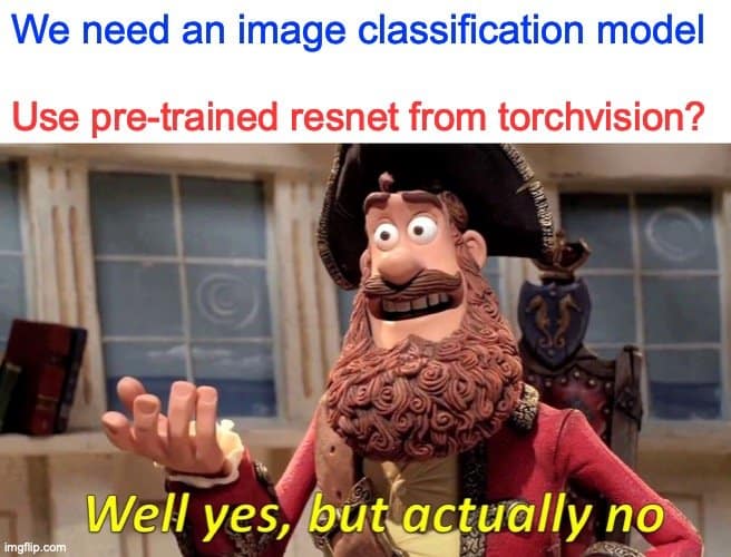
First, let’s deal with the basics. We will be using the PyTorch framework for this project. To train a style transfer model, we need a pre-trained image classification model to serve as our loss network. For keeping the computation reasonable we will use a ResNet18 model. Now that we have decided on the architecture, we need to ask ourselves, could we just use a pre-trained model from torchvision? Well yes, but actually no.
Why don’t we just use a pretrained ResNet from model zoo?
The important thing to note is that we want to run the style transfer on a webcam, with images of size 640 x 480 or even 1280 x 720 (we use 640×480 here). Most pretrained models in libraries such as torchvision or its TensorFlow equivalent are trained on imagenet at 224×224 resolution. While the architecture of ResNet18 can accept images of any size (it just does a global average pooling at the end, so all input sizes are legal), the pre-trained network has not learned useful representations of the images at that resolution.
Pretrained models behave poorly
How do we know this? Well, a ResNet18 model trained on imagenet has a top-5 classification accuracy of above 80% at 224×224. If you resize input images for a pre-trained ResNet18 to say 640×480 and perform classification at that resolution, you will find that the classification accuracy has tanked significantly. In my own experiments run on different subsets of imagenet data, I saw accuracy as low as 25%, a massive drop of 55%(!), which shows that the network isn’t really able to make sense of the features when the image resolution has changed significantly. This means that the perceptual losses calculated from such a network will not represent visual content and style information present in the images.
Knowledge Distillation (KD)
That being said, a pre-trained ResNet model is still very useful to us since the output logits from the pre-trained model (at 224×224 resolution) can be used to train a ResNet18 from scratch at 640×480 resolution. The logits can be used as ‘soft targets’ to ‘distill’ the knowledge learned by the pre-trained model. This idea of knowledge distillation (KD) was introduced by Hinton et. al. in 2015 and they showed that soft targets can help a small student network train quickly and achieve accuracy close to that of a much larger and heavier teacher network. In our case, we will use soft targets to train a model at 640×480 resolution much faster than would be possible with ‘hard targets’ or binary classification labels.
A simple explanation of KD
To understand the idea behind knowledge distillation, let’s assume there are only 3 labels in a dataset: dog, cat and bridge and we have trained a large network (say ResNet 152) on this dataset with binary labels and cross entropy loss. While training, we would have this label for a dog image:
| Label | dog | cat | bridge |
| Probability | 1 | 0 | 0 |
What is the information contained in this one-hot label? It simply states that a dog is a dog, it is neither a cat, nor a bridge. As humans we understand that while this is true, the concepts of dog and cat are somewhat close to each other in the sense that both are animals.
On the other hand, a dog is quite far away from being a bridge. In neural network speak, common features such as detecting facial hair, nose, eyes etc. would be useful in classifying dogs and cats, but not in classifying bridges. A well trained image classifier learns all this visual information and it is present in the probability vector it produces. For example, a pre-trained model might produce this distribution for a dog image:
| Label | dog | cat | bridge |
| Probability | 0.9 | 0.1 | 1e-8 |
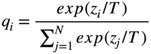
This encodes the information discussed above. So, while training a neural network, we could use the output logits from a pretrained model as targets. Since the targets are a distribution over labels and not a one-hot vector, these targets are referred to as ‘soft targets’. Mathematically, given logits zi, we can soften the targets even more by introducing a temperature factor, T in the calculation of softmax as follows:
When T=1, we recover the original softmax distribution and values higher than 1 lead to progressively softer targets. The soft targets are used to compute cross entropy loss, just as one would do with hard targets.
Advantages of using soft targets
Two points are important to note here. First, in the paper by Hinton et. al., they use a combination of both soft and hard targets while in our implementation we will only be using soft targets. Using only soft targets makes it possible to train on any set of images and not just the images for which we have labels.
The second point to note is that we will be pre-computing soft labels from a ResNet152 and storing them as a numpy array to disk. Why is this important?
Best practices of KD
Recent research by Google Brain has shown that knowledge distillation works best in practice when the teacher (ResNet152 in our case) and student (ResNet18) models process the same input views and augmentations, and when extremely long training schedules are used. In the paper, they train for 9,600 epochs! This also means that pre-computing soft labels is simple but inferior to generating them on the fly.
We will not be using these best practices to keep computation tractable and also because we don’t necessarily care about the classification accuracy of the loss network beyond a certain point. Sure, we don’t want it to be as low as 25%, but a network with 83% accuracy won’t produce dramatically different style loss than one with 80% accuracy, even though the former is clearly the better model when the application is image classification.
What does this teach us about being a successful deep learning engineer?
As a deep learning practitioner or engineer, the take home message here is that while reading research papers is important, in practice there can be many different approaches to training a network depending on the final application you care aobut. There is no one size fits all. Here, we do care about improving the accuracy of our model up from 25% to about 80%, since it is a 3x improvement but beyond that we hit the point of diminishing returns, and so we stop there since it has no perceptible bearing on our final application of style transfer. In practice, using soft targets and varying the temperature parameter from 10 down to 1, it is possible to train a ResNet18 to about 79% top-5 accuracy within 20 epochs (about 500x fewer epochs than state of the art KD recommendation!).
As a deep learning engineer working on real life projects, your success will often depend on making the best use of resources (computation, time, memory etc) to get the job done and sometimes it will require looking beyond loss metrics and academic best practices.
The Code
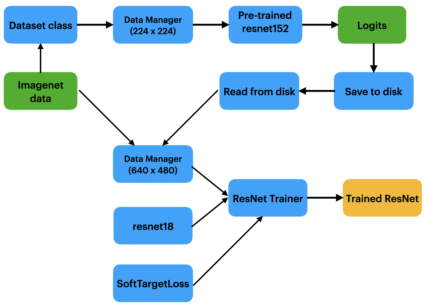
Here is the ‘plan’ we have on using different classes for training ResNet 18 on high resolution images. It is usually good to have such a plan and flowchart of a deep learning project even before we begin writing code.
Alright, enough theory. Let’s get to the code! To train ResNet18 with soft targets in PyTorch, we start by defining the DataManager class for loading data with PyTorch’s DataLoader class. This class will be useful for training the ResNet18 model as well as the final style transfer network. We will use imagenet (ILSVRC) dataset with labels for training ResNet18 and without labels for training style transfer.
import torch
from torchvision import models as models
from torch.utils.data import Dataset, DataLoader
from torchvision import transforms as T
import config as cfg
from PIL import Image
import numpy as np
import os

class ImageNetData(Dataset):
	def __init__(self, image_paths, labels=None, size=[320, 240]):
		"""
		image_paths: a list of N paths for images in training set
		labels: soft targets for images as numpy array of shape (N, 1000)
		"""
		super(ImageNetData, self).__init__()
		self.image_paths=image_paths
		self.labels=labels
		self.inputsize=size
		self.transforms=self.random_transforms()
		if self.labels is not None:
			assert len(self.image_paths)==self.labels.shape[0]
			#number of images and soft targets should be the same

	def random_transforms(self):
		normalize_transform=T.Normalize(mean=[0.485, 0.456, 0.406], std=[0.229, 0.224, 0.225])
		#define normalization transform with which the torchvision models
		#were trained

		affine=T.RandomAffine(degrees=5, translate=(0.05, 0.05))
		hflip =T.RandomHorizontalFlip(p=0.7)
		#webcam output often has horizontal flips, we would like our network
		#to be resilient to horizontal flips
		blur=T.GaussianBlur(5) #kernel size 5x5

		rt1=T.Compose([T.Resize(self.inputsize), affine, T.ToTensor(), normalize_transform])
		rt2=T.Compose([T.Resize(self.inputsize), hflip, T.ToTensor(), normalize_transform])
		rt3=T.Compose([T.Resize(self.inputsize), blur, T.ToTensor(), normalize_transform])

		return [rt1, rt2, rt3]

	def __len__(self):
		return len(self.image_paths)

	def __getitem__(self, index):
		imgpath=self.image_paths[index]
		img=Image.open(imgpath).convert('RGB')
		#some images are grayscale and need to be converted into RGB

		img_tensor=self.transforms[torch.randint(0,3,[1,1]).item()](img)

		if self.labels is None:
			return img_tensor
		else:
			label_tensor=torch.tensor(self.labels[index,:])
			return img_tensor, label_tensor

class DataManager(object):
	def __init__(self,imgpathfile, labelpath=None, size=[320, 240], use_test_data=False):
		"""
		imgpathfile: a text file containing paths of all images in the dataset
		stored as a list containting three lists for train, valid, test splits
		ex: [[p1,p2,p6...],[p3,p4...],[p5...]]

		labelpath (optional): path of .npy file which has a numpy array
		of size (N, 1000) containing pre-computed soft targets
		The order of soft targets in the numpy array should correspond to
		the order of images in imgpathfile

		size (2-list): [width, height] to which all images will be resized
		use_test_data (bool): whether or not to use test data (generally test data is used
		only once after you have verified model architecture and hyperparameters on validation dataset)
		"""

		self.imgpathfile=imgpathfile
		self.labelpath=labelpath
		self.imgsize=size

		assert os.path.exists(self.imgpathfile), 'File {} does not exist'.format(self.imgpathfile)

		self.dataloaders=self.get_data_loaders(use_test_data)

	def get_data_loaders(self, test=False):
		"""
		test (bool): whether or not to get test data loader
		"""

		with open(self.imgpathfile,'r') as f:
			train_paths, valid_paths, test_paths= eval(f.read())

		if self.labelpath is not None:
			all_labels=np.load(self.labelpath)

			assert all_labels.shape[0]== (len(train_paths)+len(valid_paths)+len(test_paths))

			train_labels=all_labels[:len(train_paths),:]
			valid_labels=all_labels[len(train_paths):len(train_paths)+len(valid_paths),:]
			test_labels=all_labels[-len(test_paths):,:]

		else:
			train_labels=None
			valid_labels=None
			test_labels=None

		train_data=ImageNetData(train_paths, train_labels, self.imgsize)
		valid_data=ImageNetData(valid_paths, valid_labels, self.imgsize)

		train_loader=DataLoader(train_data, cfg.BATCH_SIZE, shuffle=True, num_workers=cfg.NUM_WORKERS)
		valid_loader=DataLoader(valid_data, cfg.BATCH_SIZE, shuffle=True, num_workers=cfg.NUM_WORKERS)
		#evaluation of network (validation) does not require storing gradients, so GPU memory is freed up
		#therefore, validation can be performed at roughly twice the batch size of training for most
		#networks and GPUs. This reduces training time by doubling the throughput of validation

		if test:
			test_data=ImageNetData(test_paths, test_labels, self.imgsize)
			test_loader=DataLoader(test_data, cfg.BATCH_SIZE, shuffle=True, num_workers=cfg.NUM_WORKERS)

			return train_loader, valid_loader, test_loader

		return train_loader, valid_loader
There are many hyperparameters used throughout this project. It is convenient to put them all in one small config.py file so that we don’t have to dive deep into the code every time we have to make a small change during experiments.
BATCH_SIZE=64
NUM_WORKERS=8
SIZE=[480,640]
IMGPATH_FILE='./imagenetsplitpaths.txt'
SOFT_TARGET_PATH='./resnet152_results.npy'
TEMPERATURE=3
EPOCHS=10
SAVE_PATH='./resnet_{}.pt'
EVAL_INTERVAL=1000
LR=1e-4
STYLE_TARGET='./styletarget.png'
Now that we can load our data and manage hyperparameters, let us compute the soft targets from a pretrained ResNet152 model. Here we use the pretrained model provided by torchvision. For each image, the computed logits are inserted into in a numpy array and finally, the entire array is stored to disk as a .npy file. We use a text file to keep track of image paths, in order to find out which label is for which image while training the student network.
import torchvision.models as models
from dataset import DataManager
from PIL import Image
import torch
import glob
import numpy as np
import time
import config as cfg

manager=DataManager(cfg.IMGPATH_FILE, cfg.SOFT_TARGET_PATH, [224,224])


n_images=len(image_paths)

print('Inferring on {} images'.format(n_images))

device=torch.device('cuda') if torch.cuda.is_available() else torch.device('cpu')

print('Using device {}'.format(torch.cuda.get_device_name(device)))

BATCH_SIZE=256

results_152=np.zeros((n_images, 1000), dtype=np.float32)

resnet152 = models.resnet152(pretrained=True, progress=True).to(device).eval()

transform = T.Compose([T.Resize(256), T.CenterCrop(224), T.ToTensor(), T.Normalize(mean=[0.485, 0.456, 0.406],
                                 std=[0.229, 0.224, 0.225])])

begin=time.time()

for start in range(0,n_images, BATCH_SIZE):
	end= min(start+BATCH_SIZE, n_images)
	batch_names=image_paths[start:end]
	batch_images=[Image.open(p).convert('RGB') for p in batch_names]

	with torch.no_grad():
		tensor_images=[torch.unsqueeze(transform(img),0) for img in batch_images]
		in_tensor=torch.cat(tensor_images).to(device)

		out_tensor_152=resnet152(in_tensor)

		out_numpy_152=out_tensor_152.cpu().detach().numpy()

	results_152[start:end,:]=out_numpy_152

	pg=100*end/n_images
	sys.stdout.write('\r Progress= {:.2f} %'.format(pg))

np.save(f'resnet152_results.npy', results_152)

end=time.time()
print('Total time taken for inference = {:.2f}'.format(end-begin))
Once the soft targets are computed and saved to disk, we then define the Trainer class to train a student ResNet18 model, which will be used as loss network for subsequent style transfer. In addition, we define a SoftTargetLoss class, since we won’t be using the cross entropy loss provided by PyTorch.
class SoftTargetLoss(nn.Module):
	def __init__(self, temperature=1):
		"""
		Soft Target Loss as introduced by Hinton et. al.
		in https://arxiv.org/abs/1503.02531
		temp (float or int): annealing temperature hyperparameter
		temperature=1 corresponds to usual softmax
		"""
		super(SoftTargetLoss, self).__init__()
		self.register_buffer('temperature', torch.tensor(temperature))
		#temperature

	def forward(self, student_logits, teacher_logits):
		student_probabilities=nn.functional.softmax(student_logits/self.temperature)
		teacher_probabilities=nn.functional.softmax(teacher_logits/self.temperature)

		loss = - torch.mul(teacher_probabilities, torch.log(student_probabilities))

		return torch.mean(loss)
The amazing benefits of mixed precision training
One final thing to understand before we talk about the Trainer class is mixed precision training. We all know that training a network is computationally much heavier than inference and consumes more memory. The extra memory and compute required in training are used to calculate and store the gradients and update network weights.
As it turns out, for most networks the weights need not be stored in full float32 precision. Modern GPU hardware provides support for storing 16-bit floating-point parameters and performing fused multiply-accumulate (FMA) operations. Both forward and backward passes through a network can be cast into FMA operations, so having natively supported FMA ops (via tensor cores in all generations beyond Pascal) provides a massive boost to training speed without compromising on accuracy.
NVIDIA provides a handy library called apex to enable mixed-precision training in PyTorch. Using apex, mixed-precision training just requires adding 2 lines of code to achieve 2.5x speedup for ResNet18 training at O2 level optimization (recommended optimization level for most networks). This speedup was achieved on an RTX 3090. Your mileage may vary on older or less/more VRAM cards. You can check out the documentation of apex, but here is a simple summary for our purposes:
| Full Precision | Automatic Mixed precision |
model=... #define model | model=... #define model as before #add above line with opt_level |
loss=... #calculate | loss=... #same as before |
With just these two modifications to a normal PyTorch training pipeline, you can enjoy the benefits of massively improved training times and reduced memory usage. If you regularly train neural networks and have not yet implemented mixed-precision training into your pipeline, you’re missing out!
To install apex, we clone the repo and run the installation script:
git clone https://github.com/NVIDIA/apex
cd apex
pip install -v --disable-pip-version-check --no-cache-dir --global-option="--cpp_ext" --global-option="--cuda_ext" ./
Let us create the Trainer class which accepts a model and uses the DataManager class defined earlier to train the model with automatic mixed precision.
class Trainer(object):
	def __init__(self, net, manager, savepath):
		"""
		net(nn.Module): Neural network to be trained

		manager(DataManager): data manager from dataset.py

		savepath(str): a format-ready string like 'model_{}.path'
		for which .format method can be called while saving models
		at every epoch
		"""

		self.net=net
		self.manager=manager
		self.savepath=savepath #should have curly brackets, ex. 'model_{}.pth'

		self.criterion = SoftTargetLoss(cfg.TEMPERATURE)
		self.optimizer = optim.Adam(self.net.parameters(), lr=cfg.LR)
		self.writer=SummaryWriter()

	def save(self, path):
		checkpoint= {'model':self.net.state_dict(),
		'optimizer':self.optimizer.state_dict(),
		'amp':amp.state_dict() }

		torch.save(checkpoint, path)
		print(f'Saved model to {path}')

	def train(self, epochs=None, evaluate_interval=None):
		steps=0

		epochs=epochs if epochs else cfg.EPOCHS
		evaluate_interval=evaluate_interval if evaluate_interval else cfg.EVAL_INTERVAL

		device=torch.device('cuda') if torch.cuda.is_available() else torch.device('cpu')

		if device.type != 'cuda':
			print(f'GPU not found. Training will be done on device of type {device.type}')

		self.net.to(device)

		self.net, self.optimizer = amp.initialize(self.net, self.optimizer,
									opt_level='O2')

		self.net.train()

		train_iterator, valid_iterator, *_ = self.manager.dataloaders

		get_top5_accuracy=lambda p,y: (torch.topk(p, 5, dim=1).indices == torch.argmax(y, 1)[:,None]).sum(dim=1).to(torch.float).mean().item()
		mean= lambda v: sum(v)/len(v)

		for epoch in range(epochs):
			start_time=time.time()

			for idx, (x,y) in enumerate(train_iterator):
				self.optimizer.zero_grad()
				#print('Resnet input shape= ', x.shape)
				x=x.to(device)
				y=y.to(device)

				preds=self.net(x)

				loss=self.criterion(preds, y)

				#loss.backward()
				with amp.scale_loss(loss, self.optimizer) as scaled_loss:
					scaled_loss.backward()

				self.optimizer.step()

				top5_accuracy=get_top5_accuracy(preds, y)
				#this isn't *really* the top 5 accuracy because it is evaluated against the outputs of the teacher
				#model as opposed to ground truth labels. Since the value of the loss is not easy to grasp
				#intuitively, this proxy serves as an easily computable metric to monitor the progress of the
				#student network, especially if the training data is also imagenet.

				self.writer.add_scalar('Loss', loss, steps)
				self.writer.add_scalar('Top-5 training accuracy', top5_accuracy, steps)

				steps+=1

				if steps%evaluate_interval==0:
					valid_loss=[]
					valid_accuracy=[]
					self.net.eval() #put network in evaluation mode

					with torch.no_grad():
						for xv, yv in valid_iterator:
							xv=xv.to(device)
							yv=yv.to(device)
							preds=self.net(xv)
							vtop5a=get_top5_accuracy(preds, yv)

							vloss=self.criterion(preds, yv)

							valid_loss.append(vloss.item())
							valid_accuracy.append(vtop5a)

					self.writer.add_scalar('Validation Loss', mean(valid_loss), steps)
					self.writer.add_scalar('Top-5 validation accuracy', mean(valid_accuracy), steps)
					self.writer.flush()

					self.net.train() #return to training mode
					pass

			self.writer.flush() #make sure the writer updates all stats until now
			self.save(self.savepath.format(epoch))
			end_time=time.time()
			print('Time taken for last epoch = {:.3f} seconds'.format(end_time-start_time))
With this we are ready to train the ResNet18 model. We will be using a ResNet18 architecture from torchvision. We can initialize a model with the flag pretrained=False and train it with the Trainer class with the command: python3 train_resnet.py
python3 train_resnet.py
The ResNet18 model we trained at 640×480 resolution is available with the code of the blog, so if you just want to train style transfer, you should use the pre-trained model we have provided.
Implementing style transfer network
With the loss network trained, we are ready to start building the style transfer network.
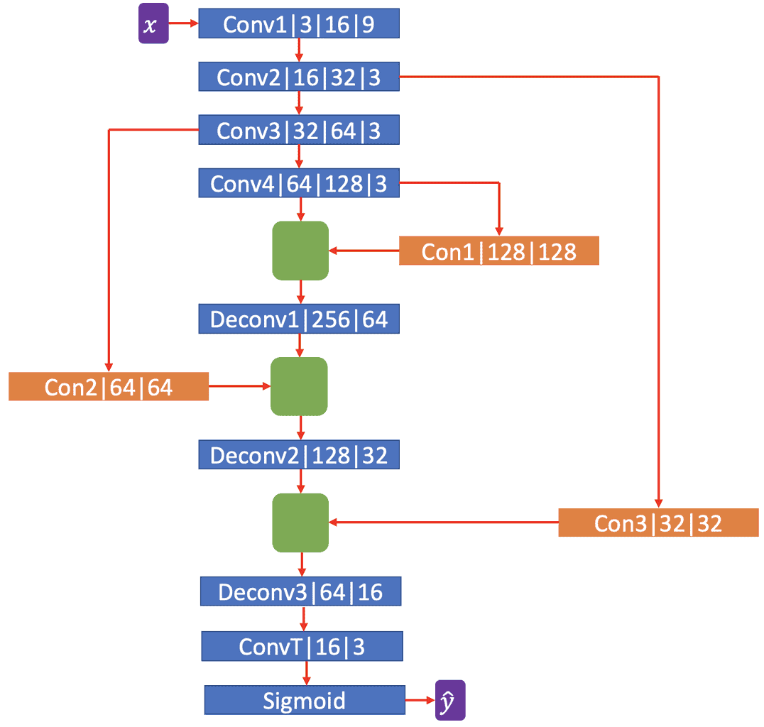
Figure 5. Architecture of the style transfer network
The architecture we are going to use is shown in figure 5. The network consists of 4 convolutional modules, Conv1 to Conv4. Each conv module consists of a convolutional layer, batch normalization layer and finally a LeakyRelu activation (with a slope of 0.1 for negative inputs). The numbers in the figure next to the module’s name represent input layers, output layers and the size of the convolution kernel respectively. After Conv4, we start upsampling the image with transposed convolution layers. However, we use two small operations to help the network generalize better.
First, we pass one of the already computed tensors from convolution modules through ‘connector modules’. Each connector module implements a depthwise separable convolution layer, such as those used in MobileNets (this was the major idea behind the original mobilenet paper). Depthwise separable convolution blocks have much fewer parameters than full convolution and are also computationally very inexpensive. All connector modules consist of depthwise separable convolution with 3×3 kernel, followed by batch norm and leaky relu. The number of input and output channels are marked in the figure next to the module name.
Second, after passing the conv tensors through connector modules, we concatenate them with outputs of conv tensors along the channel dimension, as shown in the figure with green rectangles. The network parameters are chosen so that the width and height dimensions are the same when concatenating.
After concatenating, the resulting tensors are passed through deconvolutional or transposed convolution modules. Each module consists of transposed convolution, followed by batch norm and leaky relu. Finally, there is one more transposed convolution layer with 16 input channels and 3 output channels to correspond to an RGB image. The output tensor of this layer is then passed through the sigmoid activation function to convert all pixels to a 0-1 range.
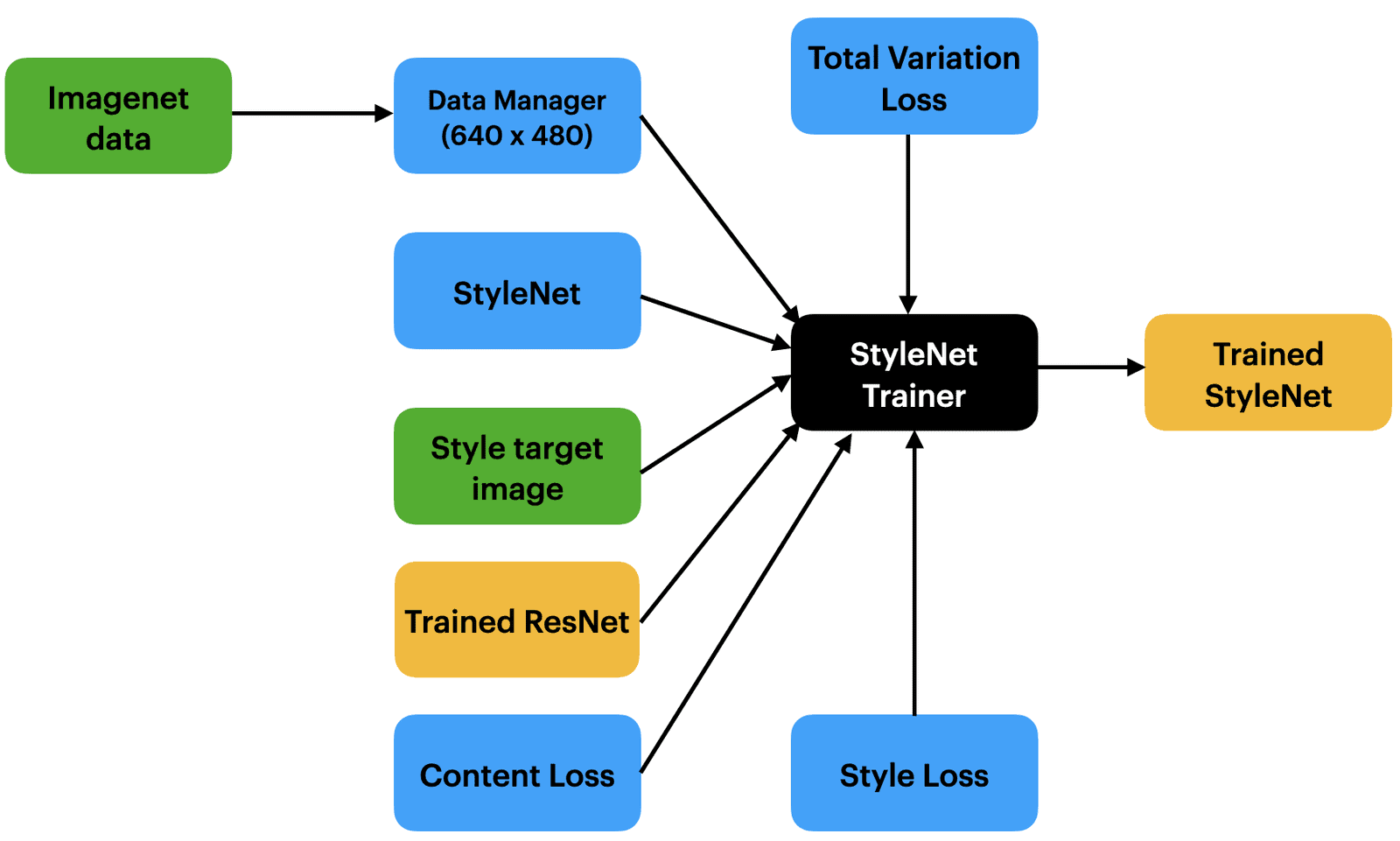
As we did in the previous section, before we dive into the code, here is a simple flowchart explaining how we plan to organize the various parts of the training pipeline.
Let us translate all these ideas into code.
import torch
import torch.nn as nn
from torch import optim
import time
import os
from PIL import Image
from torchvision import transforms as T
from torchvision import models
from torch.utils.tensorboard import SummaryWriter
from dataset import DataManager
import config as cfg
import sys

if not sys.platform=='darwin':
	from apex import amp

class StyleNetwork(nn.Module):
	def __init__(self, loadpath=None):
		super(StyleNetwork, self).__init__()
		self.loadpath=loadpath

		self.layer1 = self.get_conv_module(inc=3, outc=16, ksize=9)

		self.layer2 = self.get_conv_module(inc=16, outc=32)

		self.layer3 = self.get_conv_module(inc=32, outc=64)

		self.layer4 = self.get_conv_module(inc=64, outc=128)

		self.connector1=self.get_depthwise_separable_module(128, 128)

		self.connector2=self.get_depthwise_separable_module(64, 64)

		self.connector3=self.get_depthwise_separable_module(32, 32)

		self.layer5 = self.get_deconv_module(256, 64)

		self.layer6 = self.get_deconv_module(128, 32)

		self.layer7 = self.get_deconv_module(64, 16)

		self.layer8 = nn.ConvTranspose2d(16, 3, kernel_size=3, stride=2, padding=1, output_padding=1)

		self.activation=nn.Sigmoid()

		if self.loadpath:
			self.load_state_dict(torch.load(self.loadpath))

	def get_conv_module(self, inc, outc, ksize=3):
		padding=(ksize-1)//2
		conv=nn.Conv2d(in_channels=inc, out_channels=outc, kernel_size=ksize, stride=2, padding=padding)
		bn=nn.BatchNorm2d(outc)
		relu=nn.LeakyReLU(0.1)

		return nn.Sequential(conv, bn, relu)

	def get_deconv_module(self, inc, outc, ksize=3):
		padding=(ksize-1)//2
		tconv=nn.ConvTranspose2d(inc, outc, kernel_size=ksize, stride=2, padding=padding, output_padding=padding)
		bn=nn.BatchNorm2d(outc)
		relu=nn.LeakyReLU(0.1)

		return nn.Sequential(tconv, bn, relu)


	def get_depthwise_separable_module(self, inc, outc):
		"""
		inc(int): number of input channels
		outc(int): number of output channels

		Implements a depthwise separable convolution layer
		along with batch norm and activation.
		Intended to be used with inc=outc in the current architecture
		"""
		depthwise=nn.Conv2d(inc, inc, kernel_size=3, stride=1, padding=1, groups=inc)
		pointwise=nn.Conv2d(inc, outc, kernel_size=1, stride=1, padding=0, groups=1)
		bn_layer=nn.BatchNorm2d(outc)
		activation=nn.LeakyReLU(0.1)

		return nn.Sequential(depthwise, pointwise, bn_layer, activation)

	def forward(self, x):

		x=self.layer1(x)

		x2=self.layer2(x)

		x3=self.layer3(x2)

		x4=self.layer4(x3)

		xs4=self.connector1(x4)
		xs3=self.connector2(x3)
		xs2=self.connector3(x2)

		c1=torch.cat([x4, xs4], dim=1)

		x5=self.layer5(c1)

		c2=torch.cat([x5, xs3], dim=1)

		x6=self.layer6(c2)

		c3=torch.cat([x6, xs2], dim=1)

		x7=self.layer7(c3)

		out=self.layer8(x7)

		out=self.activation(out)

		return out
The only thing remaining now is to define the perceptual loss functions for training the network we have defined above. Here is where the ResNet18 model we trained before is used. In addition to the feature loss and style loss we explained above, we will also be using total variation (TV) loss. This loss penalizes large variations in the output image across the spatial dimensions, so having this loss encourages the network to produce relatively smooth, less choppy outputs. However, if the total variation loss is weighted significantly, the network could produce very blurry blobs, so while training we must be careful to weigh this loss appropriately. The TV loss is defined as
class TotalVariationLoss(nn.Module):
	def __init__(self):
		super(TotalVariationLoss, self).__init__()

	def forward(self, x):
		horizontal_loss=torch.pow(x[...,1:,:]-x[...,:-1,:],2).sum()

		vertical_loss=torch.pow(x[...,1:]-x[...,:-1],2).sum()

		return (horizontal_loss+vertical_loss)/x.numel()
Implementing the Style Loss
The next loss to define is style loss. The StyleLoss module accepts features of both style target image and input image. It computes the gram matrices corresponding to features of both the images and computes the mean squared error between the two gram matrices.
class StyleLoss(nn.Module):
	def __init__(self):
		super(StyleLoss, self).__init__()
		pass

	def forward(self, target_features, output_features):

		loss=0

		for target_f,out_f in zip(target_features, output_features):
			#target is batch size 1
			t_bs,t_ch,t_w,t_h=target_f.shape
			assert t_bs ==1, 'Network should be trained for only one target image'

			target_f=target_f.reshape(t_ch, t_w*t_h)

			target_gram_matrix=torch.matmul(target_f,target_f.T)/(t_ch*t_w*t_h) #t_ch x t_ch matrix

			i_bs, i_ch, i_w, i_h = out_f.shape

			assert t_ch == i_ch, 'Bug'

			for img_f in out_f: #contains features for batch of images
				img_f=img_f.reshape(i_ch, i_w*i_h)

				img_gram_matrix=torch.matmul(img_f, img_f.T)/(i_ch*i_w*i_h)

				loss+= torch.square(target_gram_matrix - img_gram_matrix).mean()

		return loss
Implementing the Content Loss
Finally, the content loss as explained earlier, just simply computes the mean squared error between the features of the stylized image y and x.
class ContentLoss(nn.Module):
	def __init__(self):
		super(ContentLoss, self).__init__()

	def forward(self, style_features, content_features):
		loss=0
		for sf,cf in zip(style_features, content_features):
			a,b,c,d=sf.shape
			loss+=(torch.square(sf-cf)/(a*b*c*d)).mean()

		return loss
Now, we are ready to write the Trainer class for training Style transfer network. As explained above, we will use automatic mixed precision to speed up training. AMP is a bit tricky when two networks are involved, but we will keep the loss network completely out of the scope of AMP. This reduces the speedup we can obtain at O2 level, but is easier to follow and there is no scope of introducing bugs due to unintended updating of the parameters of the loss network. The Trainer class then looks like this
class StyleTrainer(object):
	def __init__(self, student_network, loss_network, style_target_path, data_manager,feature_loss, style_loss, savepath=None):
		self.student_network=student_network
		self.loss_network=loss_network

		assert os.path.exists(style_target_path), 'Style target does not exist'
		image=Image.open(style_target_path).convert('RGB').resize(cfg.SIZE[::-1])
		preprocess=T.Compose([T.ToTensor(), T.Normalize(mean=[0.485, 0.456, 0.406], std=[0.229, 0.224, 0.225])])

		self.style_target=torch.unsqueeze(preprocess(image),0)

		self.manager=data_manager

		self.feature_loss=feature_loss

		self.style_loss=style_loss

		self.total_variation = TotalVariationLoss()

		self.savepath=savepath

		self.writer=SummaryWriter()

		self.optimizer=optim.Adam(self.student_network.parameters(), lr=cfg.LR)

	def train(self, epochs=None, eval_interval=None, style_loss_weight=1.0):
		pass
		epochs= epochs if epochs else cfg.EPOCHS
		eval_interval=eval_interval if eval_interval else cfg.EVAL_INTERVAL

		device = torch.device('cuda') if torch.cuda.is_available() else torch.device('cpu')
		train_loader, valid_loader, *_ = self.manager.dataloaders #ignore test loader if any

		self.student_network.to(device).train()

		self.loss_network.to(device)
		self.loss_network.eval()

		self.student_network, self.optimizer = amp.initialize(self.student_network, self.optimizer,
									opt_level='O2', enabled=True)

		self.style_target=self.style_target.to(device)

		style_target_features=resnet_forward(self.loss_network,self.style_target) #fixed during training

		step=0

		for epoch in range(epochs):
			estart=time.time()
			for x in train_loader:
				self.optimizer.zero_grad()

				x=x.to(device)

				stylized_image = self.student_network(x)
				content_features = resnet_forward(self.loss_network, x) #self.loss_network(x)
				stylized_features= resnet_forward(self.loss_network, stylized_image)#self.loss_network(stylized_image)

				feature_loss=self.feature_loss(stylized_features, content_features)

				style_loss=self.style_loss(style_target_features, content_features)

				tvloss=self.total_variation(stylized_image)

				loss = 1000*feature_loss + style_loss_weight*style_loss + 0.02*tvloss

				self.writer.add_scalar('Feature loss', feature_loss.item(), step)
				self.writer.add_scalar('Style loss', style_loss.item(), step)
				self.writer.add_scalar('Total Variation Loss', tvloss.item(), step)

				#loss.backward()
				with amp.scale_loss(loss, self.optimizer) as scaled_loss:
					scaled_loss.backward()

				self.optimizer.step()

				step+=1

				if step%eval_interval==0:
					self.student_network.eval()

					with torch.no_grad():
						pass
						for imgs in valid_loader:
							imgs=imgs.to(device)
							stylized=self.student_network(imgs)
							self.writer.add_images('Stylized Examples', stylized, step)
							break #just one batch is enough

					self.student_network.train()

			self.save(epoch)
			eend=time.time()
			print('Time taken for last epoch = {:.3f}'.format(eend-estart))

	def save(self, epoch):
		if self.savepath:
			path=self.savepath.format(epoch)
			torch.save(self.student_network.state_dict(), path)
			print(f'Saved model to {path}')
The training loop for style transfer network can now be written with minimal code. Here, as a good programming practice, we explicitly set the ‘requires_grad’ flag of every parameter of the loss network to False.
if __name__=="__main__":
	net=StyleNetwork()
	manager=DataManager(cfg.IMGPATH_FILE, None, cfg.SIZE) #Datamanager without soft targets
	styleloss=StyleLoss()
	contentloss=ContentLoss()
	loss_network= models.resnet18()
	loss_network.load_state_dict(torch.load('./models/resnet_9.pt')['model'])

	for p in loss_network.parameters():
		p.requires_grad=False #freeze loss network

	trainer=StyleTrainer(net, loss_network,cfg.STYLE_TARGET, manager, contentloss, styleloss, './style_{}.pth')
	trainer.train()
Now, it’s time to train the style transfer model!
python3 stylenet.py
The trained model is saved as a .pth file and we can now begin the exciting process of using this model in our Zoom call.
Creating a virtual camera
We will cover two ways of creating a virtual camera. The first one works only on Linux and teaches us a lot about the kernel modules in Linux. The second method works on all operating systems Linux, Windows and macOS.
Linux only method
Linux is quite amazing in that it allows the user to add and remove modules from the operating system. We will use a module called v4l2loopback. As the name implies, this module can be used to create virtual v4l2 devices which can be written to. The input to the device is looped back to the output.
Since this is a kernel module, there aren’t any dependencies as such. To install this module, we clone a GitHub repository, make and install the module and to use the module, we load the module using modprobe.
git clone https://github.com/umlaeute/v4l2loopback
cd v4l2loopback
make
sudo make install
In case you are running the model training and inference in a docker container, you can pass the virtual device created as an argument while launching the container with –device flag and write to it from within the container. v4l2loopback works flawlessly and the virtual camera will show the frames written from inside the container into the Zoom meeting created in the main machine.
This method has the great advantage that any number of virtual devices can be created. You can do all sorts of funky stuff like reading from one real camera and writing to two virtual cameras so that you can log into two meetings, say one with Zoom and another with Skype/Slack/Teams, which is not possible with one real camera. Moreover, this method will also work on embedded boards like NVIDIA Jetson line of boards which don’t have officially supported binaries for OBS.
General method (Windows/macOS, Linux)
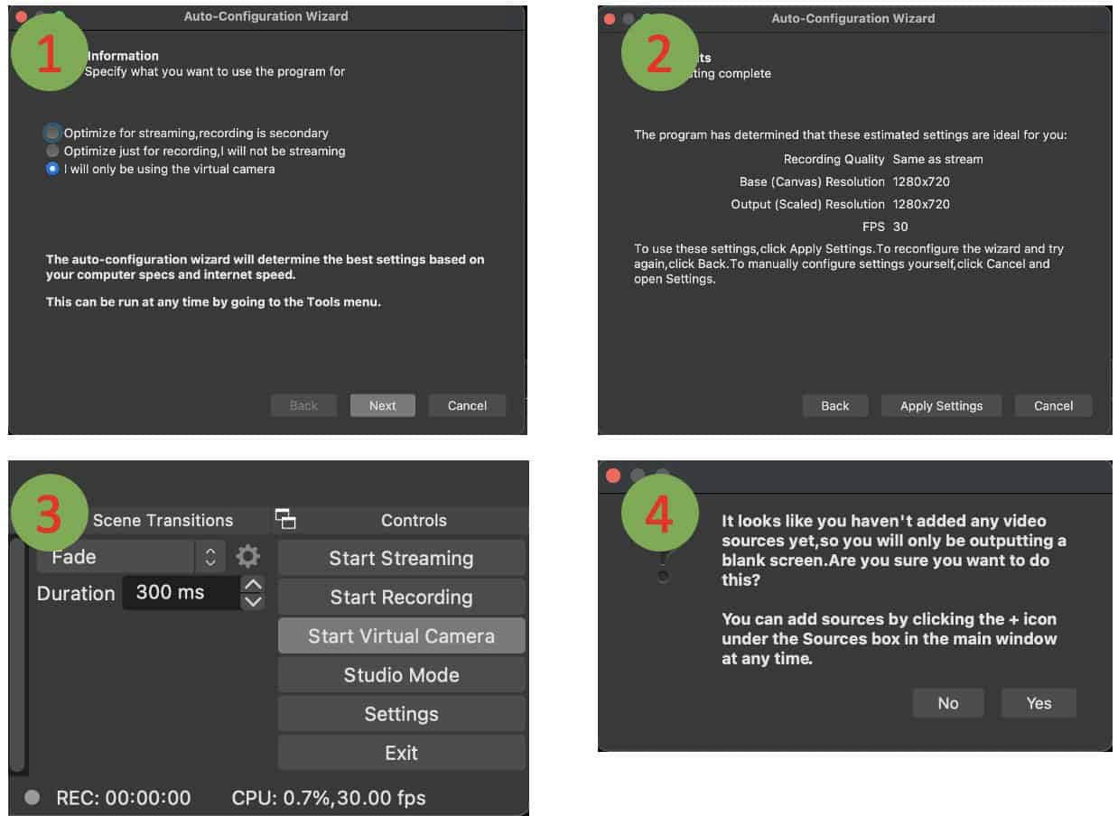
Open Broadcaster Software (OBS) is a software for streaming to YouTube/Twitch and many other streaming platforms and is very popular among gamers. OBS works on all operating systems. The important part for us is that OBS can create a virtual camera which can be written to via a python script and read from by Zoom/Skype etc. To get started, download the OBS installer for your operating system of choice and install it by following the steps shown in the installer. When you open OBS for the first time, you should follow the steps explained in figure 4. In the configuration window, select “I will only be using the virtual camera” and click Next. Then click Apply Settings. Next, in the OBS window on the bottom right corner, click on ‘Start Virtual Camera’. A warning window will appear stating that a blank window will be shown. This is okay for now, so just click Yes. Once this is done, you can close the OBS app. The camera has been created and will now be visible to the network inference script we are going to write next.
Running style transfer in a Zoom meeting
On Linux via ffmpeg
Ffmpeg is the swiss army knife of video/audio processing. If you regularly work with videos or audio and are not yet familiar with ffmpeg, you are really missing out. I promise that any time spent in learning how to use ffmpeg will be fruitful and will save you tons of time and frustration. Assuming that you installed v4l2loopback and created a virtual camera as explained in the Linux specific section above, the general strategy we will now use is to create an ffmpeg pipeline. This pipeline reads frame data from standard input and encodes it into a format that is compatible with v4l2 cameras. The converted frame data is written to the virtual v4l2 device we created above.
The ffmpeg pipeline reads:
ffmpeg -re -f rawvideo -pix_fmt rgb24 -s 640x480 -i - -f v4l2 -pix_fmt yuv420p /dev/video2
If the above line seems mysterious and unintelligible to you at the moment, don’t worry. In complicated ffmpeg pipelines, I have often found the ‘hey, ffmpeg’ method to be very useful in creating and debugging ffmpeg pipelines. Let us color code every part of the pipeline and break down the statement with this method:
You can read this as,

The device /dev/video2 was the virtual device created with v4l2loopback in this case. You should use the device number created on your machine. Each of the above parameters is carefully chosen, such as the frame size, input pixel format, standard input data source, yuv420p pixel format and finally the device number.
You can change the size parameter if you train the network for a different resolution, but the pixel format for v4l2 device should not be changed because Zoom understands raw frame data only in yuv420p format and will not accept, for example, rgb24 format. The above ffmpeg pipeline is the crux of the inference script.
With this understood, the rest of the inference script is quite straight forward. You will need to connect a real USB camera to your linux computer. We will use opencv to read live video frames from this camera, pass them through the trained style transfer network and convert the output of the neural network into a numpy array of unsigned 8-bit integer type. This data, which is in rgb24 format, is written to the standard input of the ffmpeg subprocess. Ffmpeg converts this data into yuv420p format and writes it to the virtual camera device.
import cv2
import numpy as np
import subprocess
import torch
from stylenet import StyleNetwork
from torchvision import transforms as T

net=StyleNetwork('./models/style_7.pth')

for p in net.parameters():
	p.requires_grad=False

device=torch.device('cuda') if torch.cuda.is_available() else torch.device('cpu')

net=net.eval().to(device) #use eval just for safety

src=cv2.VideoCapture('/dev/video0') #USB camera ID

ffstr='ffmpeg -re -f rawvideo -pix_fmt rgb24 -s 640x480 -i - -f v4l2 -pix_fmt yuv420p /dev/video2'
#ffmpeg pipeline which accepts raw rgb frames from command line and writes to virtul camera in yuv420p format

zoom=subprocess.Popen(ffstr, shell=True, stdin=subprocess.PIPE) #open process with shell so we can write to it

dummyframe=255*np.ones((480,640,3), dtype=np.uint8) #blank frame if camera cannot be read

preprocess=T.Normalize(mean=[0.485, 0.456, 0.406], std=[0.229, 0.224, 0.225])
#same normalization as that used in training data

ret, frame=src.read()

while True:
	try:
		if ret:
			frame=(frame[:,:,::-1]/255.0).astype(np.float32) #convert BGR to RGB, convert to 0-1 range and cast to float32
			frame_tensor=torch.unsqueeze(torch.from_numpy(frame),0).permute(0,3,1,2)
			# add batch dimension and convert to NCHW format

			tensor_in = preprocess(frame_tensor) #normalize
			tensor_in=tensor_in.to(device) #send to GPU

			tensor_out = net(tensor_in) #stylized tensor
			tensor_out=torch.squeeze(tensor_out).permute(1,2,0) #remove batch dimension and convert to HWC (opencv format)
			stylized_frame=(255*(tensor_out.to('cpu').detach().numpy())).astype(np.uint8) #convert to 0-255 range and cast as uint8
		else:
			stylized_frame=dummyframe #if camera cannot be read, blank white image will be shown

		zoom.stdin.write(stylized_frame.tobytes())
		#write to ffmpeg pipeline which in turn writes to virtual camera that can be accessed by zoom/skype/teams

		ret,frame=src.read()
	except KeyboardInterrupt:
		print('Received stop command')
		break

zoom.terminate()
src.release() #close ffmpeg pipeline and release camera
You can run this script with
python3 livedemo.py
Now, when you join a Zoom meeting, you should now see the option to use virtual camera and once you have chosen it, the stylized video will be shown to others in the meeting as your camera feed. Congratulations!
On Windows/Mac via pyvirtualcam
On Mac or Windows, we can let a library called pyvirtualcamera do everything for us. It makes life easier and the code looks clean but you also miss out on the opportunity to learn intricacies of tools like ffmpeg (on Linux, pyvirtualcamera uses ffmpeg and v4l2loopback under the hood, just like we did). The basic process is the same. Once the virtual camera has been created (using OBS), we read live video feed from a real camera, convert it to stylized frame by passing it through the trained style transfer network, and write it to the virtual camera. The part related to inference is exactly the same as before
import pyvirtualcam
import numpy as np
import cv2
import torch
from stylenet import StyleNetwork
from torchvision import transforms as T


net=StyleNetwork('./models/style_7.pth')

for p in net.parameters():
    p.requires_grad=False

device=torch.device('cuda') if torch.cuda.is_available() else torch.device('cpu')

net=net.eval().to(device) #use eval just for safety

src=cv2.VideoCapture(0) #USB camera ID

preprocess=T.Normalize(mean=[0.485, 0.456, 0.406], std=[0.229, 0.224, 0.225])
#same normalization as that used in training data

ret, frame=src.read()

with pyvirtualcam.Camera(width=640, height=480, fps=20) as vcam:

    print(f'Using virtual camera: {cam.device} at {cam.width} x {cam.height}')

    while True:
        try:
            if ret:
                frame=(frame[:,:,::-1]/255.0).astype(np.float32) #convert BGR to RGB, convert to 0-1 range and cast to float32
                frame_tensor=torch.unsqueeze(torch.from_numpy(frame),0).permute(0,3,1,2)
                # add batch dimension and convert to NCHW format

                tensor_in = preprocess(frame_tensor) #normalize
                tensor_in=tensor_in.to(device) #send to GPU

                tensor_out = net(tensor_in) #stylized tensor
                tensor_out=torch.squeeze(tensor_out).permute(1,2,0) #remove batch dimension and convert to HWC (opencv format)
                stylized_frame=(255*(tensor_out.to('cpu').detach().numpy())).astype(np.uint8) #convert to 0-255 range and cast as uint8
            else:
                stylized_frame=dummyframe #if camera cannot be read, blank white image will be shown

            vcam.send(stylized_frame)
            #write to ffmpeg pipeline which in turn writes to virtual camera that can be accessed by zoom/skype/teams

            ret,frame=src.read()

        except KeyboardInterrupt:
            print('Received stop command')
            break

src.release() #close ffmpeg pipeline and release camera
Now, when you join a Zoom meeting you should see ‘OBS Virtual Camera’ in the list of devices. Select it and the inference from neural network will be shown as your camera feed to others in the meeting! Congratulations!
Summary
If you have reached this far, you should congratulate yourself. This was a long post and we covered many different concepts like
- basics of neural style transfer proposed by Gatys et. al.,
- a more advanced real time algorithm proposed by Johnson et. al.,
- automatic mixed precision training with NVIDIA apex,
- knowledge distillation proposed by Hinton et. al.,
- Training a ResNet at high resolution (and importantly why we did it!)
- coding up a style transfer network in PyTorch,
- implementing the three types of loss functions (content loss, style loss, total variation loss),
- creating virtual cameras in Linux and Windows/Mac,
- v4l2loopback,
- Some basics of ffmpeg,
- Inference of trained network on a live camera feed and finally
- Enjoying an interesting web meeting
From here on, you can take this even further since any type of neural network can be incorporated into your Zoom meeting. For example, you could demonstrate image classification, or live object detection, or live semantic segmentation or optical flow all with the same approach. This, therefore, can become an exciting and hands-on way to learn and teach computer vision algorithms in general. We share our results with style transfer in the video below.










100K+ Learners
Join Free OpenCV Bootcamp3 Hours of Learning