In our previous blog we learnt how to install the libpytorch libraries and run the pytorch C++ frontend application. If you have not read that yet, here is the link to Part-1/1 <give link to previous blog>
In this blog, instead of diving right away in to coding, for the benefit of all, We will split this tutorial in to two parts
- Part 2.1 – Crash course on the basics.
- Part 2.2 – Building Neural nets using C++
If you already know the bascis of neural net, you should have no problem in understanding the Part-2.2 without reading the content in Part-2.1. We try to keep it short and interesting by trying to visualize the equations via animated gifs. But please note that we write all the code based on the terms and variables which we introduced while explaining the concepts in Part-2.1.
Part 2.1: Crash course on the basics
There are plenty of material available online about the basics of Neural net including a blog in learnopencv.com. If you enjoy to learn by watching videos, then we recommend you to watch the MIT course video lectures on the topic. Most of the illustrations and examples we build in this blog will be straight out of those lectures.
We assume you have some prior knowledge on the concepts and we do not get in to the nitty gritty details of mathematics in this blog.
Prof Patrick Winston has done a wonderful job of explaining the concepts in its simpletst form in the MIT lecture videos. We just give you a high level equations which we require to implement as python and C++ code.
NOTE: Througout this blog we try to get the visual intuition to the equations which we arrive at. Rather than writing too much text about the equation itself.
Perceptrons:
We know that typically neurons are the weighted sums of inputs. Each unit has some number of weighted inputs. These weighted inputs are summed together (a linear combination) then passed through an activation function to get the unit’s output.

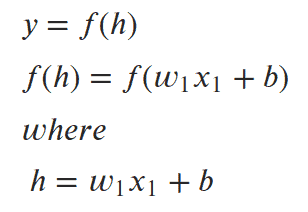
Let us write the mathematical formual for our above illustration.

If you pay attention to the equation involving “h” you notice something interesting. It looks very similar to the equation y = mx + b. Which is an equation of straight line!
To solidify our understanding, let us visualize the network with two input elements.

Similar to Equation 1. We can write the equation for two input perceptron as Equation 2 as shown below.

We can also generalize Eqation 2 for “m” number of inputs as follows.

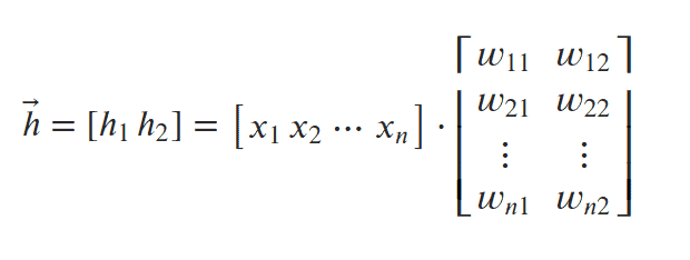
Equation 3 is called system of linear equations. We can represent the system of linear equations in Matrix form as shown below (Equation 4). We can solve these equations as dot product of two matrices.

Activation Function:
So far we only concentrated on the value of “h” in the above equations. Let us zoom in a bit on the function “f(h)” and understand what it does. The function f(h) is called the Activation function .

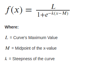
There are different types of activation functions available. For the purpose of illustrations, in this blog we stick with “Sigmoid Function“.

Here is a quick look at how the sigmoid curve behaves for different values of k and M.

Part 2.2: Building Neural nets using C++
With this much of basic information about the input, weights, bias and activation function, we can start writing the code for our Neural network.
Activation Function:
Here is the code for Sigmoid activation function in its simplest form.
Python Code:
import torch

def ActivationFunction(x):
    """ Sigmoid activation function

        Arguments
        ---------
        x: torch.Tensor
    """
    return 1/(1+torch.exp(-x))
C++ Code:
#include<torch/torch.h>
#include<ATen/Context.h>
#include<iostream>

torch::Tensor ActivationFunction(const torch::Tensor& x)
{
  // Sigmoid function.
  auto retVal = 1/(1+torch::exp(-x));
  return retVal;
}
We can see that torch::exp() in C++ is equivalent of torch.exp() in python code. There is nothing complicated in the above code, we are just implementing the sigmoid equation.
To build a network we need inputs (x), weights (w) and bias (b). Initially all the values which we chose are random. From our previous blog, we already know how to generate random normally distributed numbers.
Python Code:
### Generate some data

# Set the random seed to keep the output reproducible.
torch.manual_seed(3)

# input units are called features. Let us have 7 of them.
features = torch.randn((1, 7))

# Weights for our data.
weights = torch.randn_like(features)

# and the bias terms.
bias = torch.randn((1, 1))
C++ Code:
int main()
{
  torch::manual_seed(3);

  // input : x
  torch::Tensor features = torch::randn({1, 7});

  // weight : w
  auto weights = torch::randn_like(features);

  // bias : b
  auto bias = torch::randn({1,1});
}
By observing the highlighted code above; we note that, both python and C++ has similar set of API’s. Also notice that we are using torch::randn() instead of torch::rand().
torch::randn() returns a tensor filled with random numbers from a normal distribution with mean ‘0’ and variance ‘1’ (also called the standard normal distribution).
torch::randn_like() returns a tensor with the same size as input that is filled with random numbers from a uniform distribution in the interval [0, 1).
PyTorch tensors can be added, multiplied, subtracted, etc, just like Numpy arrays. In general, you’ll use PyTorch tensors pretty much the same way you would use Numpy arrays. Let us use the generated data to calculate the output of this simple single layer network.
Python Code:
We use the sigmoid activation function, which we wrote earlier.
y = ActivationFunction(torch.sum(features * weights) + bias)

y = ActivationFunction((features * weights).sum() + bias)

y = ActivationFunction(torch.mm(features, weights.view(7,1)) + bias)
C++ Code:
Similar to python, there are multiple ways to get the same result in C++. Here are few options.
torch::sum(features * weights)
(features * weights).sum()
torch::mm(features, weights.view({7,1}))
In general, you want to use torch::mm() since they are more efficient and accelerated using modern libraries and high-performance computing on GPUs.
We should note that, we need to reshape the tensor while using tensor::mm(). We can use view() or reshape() or resize_() methods as discussed in our previous blog to reshape the pytorch tensors.
Using .reshape() to reshpae the tensor.
torch::mm(features, weights.reshape({7,1}))
Using .resize_() to reshape the tensor. In pytorch whenever we see an API with “_” (under_score) then those operations are done inplace. Pytorch python version of under_score API’s are also available in pytorch C++ frontend libraries.
torch::mm(features, weights.resize_({7,1})
As previously mentione we prefer using .view().
torch::mm(features, weights.view({7,1})
Putting it all together.
#include <torch/torch.h>
#include <ATen/Context.h>
#include <iostream>

torch::Tensor ActivationFunction(const torch::Tensor &x)
{
  // Sigmoid function.
  auto retVal = 1/(1+torch::exp(-x));
  return retVal;
}

int main()
{
  torch::manual_seed(3);

  torch::Tensor features = torch::randn({1, 7});

  auto weights = torch::randn_like(features);

  auto bias = torch::randn({1,1});

  y = ActivationFunction(torch::mm(features, weights.view({7,1}))+bias);

  return 0;
}
Congratulations! you just built your own single neuron from scratch using pytorch C++ frontend libraries!
Stacked Neural Net:
Unfortunately single neuron is of no use for us. The real power of this algorithm can be harnessed only when we start stacking these individual units into layers and stack these layers, into a network of neurons. The output of one layer of neuron becomes the input for the next layer.
With multiple input and output units, let us see how we can express the weights as a matrix.

Here is the mathematical expression for the hidden layer ℎ1 and ℎ2.

Hopefully illustration of the above stacked Neural net gives better intution about how the matrix with values W11, W12, W13, …. Wn1, Wn2 being used in forming a weight matrix.
One thing to note is that, here we are connecting all the input nodes with all the hidden nodes. And all the hidden nodes are in turn connected to all the nodes in the output layer. This is common while setting up the initial network. This could cause the network to “Overfit” our model. To avoid overfitting, a popular method called dropout is used.
In simple terms, process of dropping few connections from one layer to another is called dropout. Later while implementing the CNN model for MNIST and CIFAR-10, we will see how to implement the dropout programmatically using C++ frontend API’s.
Ideally there will be one input and one output layer with many hidden layers will be there in a network. In general, more the number of hidden layers more complex your network is. With this much information we are ready to build our first Stacked neural net.
Here is the gist of our Stacked neural net. which comes handy while we write the code.
- Number of input Layers = 1
- Number hidden layers = 1
- Number of output layers = 1
- Number of input units = 3 (i.e. X1, X2, X3)
- Number of hidden units in the hidden layer = 2 (i.e h1 & h2)
- Number of units in the output layer = 1 (i.e. y).
- If we are building Cats and Dogs classifier then number of output units will be 2. Similarly, if we are building MNIST digits classifier then number of output units will be 10 (digits 0 – 9) so on and so forth.
As usual we will take a python implementation of our stacked network as example and write the equivalent network in C++.
Python Code:
# Set the random seed to get reproducible results.
torch.manual_seed(7)

#  number of input units = 3.
features = torch.randn((1, 3))

# Define the size of each layer in our network
n_input = features.shape[1]
n_hidden = 2
n_output = 1

# Weights for inputs to hidden layer
W1 = torch.randn(n_input, n_hidden)
# Weights for hidden layer to output layer
W2 = torch.randn(n_hidden, n_output)

# and bias terms for hidden and output layers
B1 = torch.randn((1, n_hidden))
B2 = torch.randn((1, n_output))

# Feeding one neural network output with other. aka stacking.
h = ActivationFunction(torch.mm(features, W1) + B1)
output = ActivationFunction(torch.mm(h, W2) + B2)
print(output)
C++ Code:
We have three input units in our input layer (X1, X2, X3), hence we create a 1 * 3 (1 row and 3 column) tensor of random numbers
  // Seed for Random number
  torch::manual_seed(9);

  torch::Tensor features = torch::randn({1, 3});
Define the size of each layer in our network. Number of input units, must match number of input features
auto num_inputs = features.size(1);
Number of hidden units
int num_hidden_units = 2;
Number of output units
int num_output = 1;
Weights for inputs to hidden units
  auto W1 = torch::randn({num_inputs, num_hidden_units});

  auto W2 = torch::randn({num_hidden_units, num_output});
and bias terms for hidden and output layers. Always pay special attention to the dimensions of the tensors which you are creating. The dimensions of rows and columns should match while passing it from one layer to the other.
  auto B1 = torch::randn({1, num_hidden_units});

  auto B2 = torch::randn({1, num_output});
Finally pass the input of one layer in to the other. In other words stack the layers. Notice that variable “h” is being passed as an input to the variable “y“
auto h = ActivationFunction(torch::mm(features, W1) + B1);

auto y = ActivationFunction(torch::mm(h, W2) + B2);
Finally putting it all at one place. Our neural net looks as follows.
#include <torch/torch.h>
#include <ATen/Context.h>
#include <iostream>

torch::Tensor ActivationFunction(const torch::Tensor &x)
{
  // Sigmoid function.
  auto retVal = 1/(1+torch::exp(-x));
  return retVal;
}


int main()
{
  // Seed for Random number
  torch::manual_seed(9);

  torch::Tensor features = torch::rand({1, 3});
  //auto features = torch::rand({1, 3});
  std::cout << "features = " << features << "\n";

  // Define the size of each layer in our network
  // Number of input units, must match number of input features
  auto num_inputs = features.size(1);
  // Number of hidden units
  int num_hidden_units = 2;
  // Number of output units
  int num_output = 1;


  // Weights for inputs to hidden layer
  auto W1 = torch::randn({num_inputs, num_hidden_units});
  std::cout << "W1 = " << W1.sizes() << "\n";
  // Weights for hidden layer to output layer
  auto W2 = torch::randn({num_hidden_units, num_output});
  std::cout << "W2 = " << W2.sizes() << "\n";

  // and bias terms for hidden and output layers
  auto B1 = torch::randn({1, num_hidden_units});
  std::cout << "B1 = " << B1.sizes() << "\n";
  auto B2 = torch::randn({1, num_output});
  std::cout << "B2 = " << B2.sizes() << "\n";


  auto h = ActivationFunction(torch::mm(features, W1) + B1);
  auto y = ActivationFunction(torch::mm(h, W2) + B2);
  std::cout << "y = " << y << "\n";
  return 0;
}
Note that we are not doing any training on the network yet. In our next blog we will see how to do training and testing of our network on MNIST data set.


