In this post, we will learn about Principal Component Analysis (PCA) — a popular dimensionality reduction technique in Machine Learning. Our goal is to form an intuitive understanding of PCA without going into all the mathematical details.
At the time of writing this post, the population of the United States is roughly 325 million. You may think millions of people will have a million different ideas, opinions, and thoughts, after all, every person is unique. Right?
Wrong!
Humans are like sheep. We follow a herd. It’s sad but true.
Let’s say you select 20 top political questions in the United States and ask millions of people to answer these questions using a yes or a no. Here are a few examples
1. Do you support gun control?
2. Do you support a woman’s right to abortion?
And so on and so forth. Technically, you can get ![]() different answers sets because you have 20 questions and each question has to be answered using a yes or a no.
different answers sets because you have 20 questions and each question has to be answered using a yes or a no.
In practice, you will notice the answer set is much much smaller. In fact, you replace the top 20 questions with a single question
“Are you a democrat or a republican?”
and accurately predict the answer to the rest of the questions with a high degree of accuracy. So, this 20-dimensional data is compressed to a single dimension and not much information is lost!
This is exactly what PCA allows us to do. In a multi-dimensional data, it will help us find the dimensions that are most useful and contain the most information. It will help us extract essential information from data by reducing the dimensions.
We will need some mathematical tools to understand PCA and let’s begin with an important concept in statistics called the variance.
What is variance?
The variance measures the spread of the data. In Figure 1 (a), the points have a high variance because they are spread out, but in Figure 1 (b), the points have a low variance because they are close together.

Also, note that in Figure 1 (a) the variance is not the same in all directions. The direction of maximum variance is especially important. Let’s see why.
Why do we care about the direction of maximum variance?
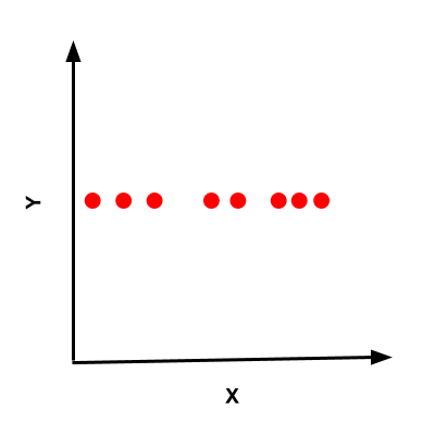
Variance encodes information contained in the data. For example, if you had 2D data represented by points with ![]() coordinates. For n such points, you need 2n numbers to represent this data. Consider a special case where for every data point the value along the y-axis was 0 (or constant). This is shown in Figure 2
coordinates. For n such points, you need 2n numbers to represent this data. Consider a special case where for every data point the value along the y-axis was 0 (or constant). This is shown in Figure 2
It is fair to say that there is no (or very little) information along the y-axis. You can compactly represent this data using n numbers to represent its value along the x-axis and only 1 common number to represent the constant along the y-axis. Because there is more variance along the x-axis, there is more information, and hence we have to use more numbers to represent this data. On the other hand, since there is no variance along the y-axis, a single number can be used to represent all information contained in n points along this axis.
What is Principal Component Analysis
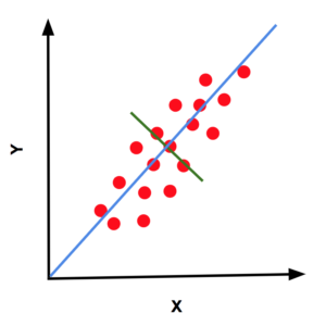
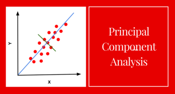
Now consider a slightly more complicated dataset shown in Figure 3 using red dots. The data is spread in a shape that roughly looks like an ellipse. The major axis of the ellipse is the direction of maximum variance and as we know now, it is the direction of maximum information. This direction, represented by the blue line in Figure 3, is called the first principal component of the data.
The second principal component is the direction of maximum variance perpendicular to the direction of the first principal component. In 2D, there is only one direction that is perpendicular to the first principal component, and so that is the second principal component. This is shown in Figure 3 using a green line.
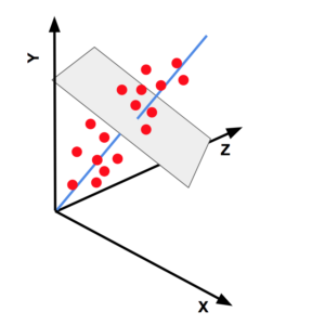
Now consider 3D data spread like an ellipsoid (shown in Figure 4). The first principal component is represented by the blue line. There is an entire plane that is perpendicular to the first principal component. Therefore, there are infinite directions to choose from and the second principal component is chosen to be the direction of maximum variance in this plane. As you may have guessed, the third principal component is simply the direction perpendicular to both the first and second principal components.
PCA and Dimensionality Reduction
In the beginning of this post, we had mentioned that the biggest motivation for PCA is dimensionality reduction. In other words, we want to capture information contained in the data using fewer dimensions.
Let’s consider the 3D data shown in Figure 4. Every data point has 3 coordinates – x, y, and z which represent their values along the X, Y and Z axes. Notice the three principal components are nothing but a new set of axes because they are perpendicular to each other. We can call these axes formed by the principal components X’, Y’ and Z’.
In fact, you can rotate the X, Y, Z axes along with all the data points in 3D such that the X-axis aligns with the first principal component, the Y-axis aligns with the second principal component and the Z-axis aligns with the third principal components. By applying this rotation we can transform any point (x, y, z) in the XYZ coordinate system to a point (x’, y’, z’) in the new X’Y’Z’ coordinate system. It is the same information presented in a different coordinate system, but the beauty of this new coordinate system X’Y’Z’ is that the information contained in X’ is maximum, followed by Y’ and then Z’. If you drop the coordinate z’ for every point (x’, y’, z’) we still retain most of the information, but now we need only two dimensions to represent this data.
This may look like a small saving, but if you have 1000 dimensional data, you may be able to reduce the dimension dramatically to maybe just 20 dimensions. In addition to reducing the dimension, PCA will also remove noise in the data.
What are Eigen vectors and Eigen values of a matrix?
In the next section, we will explain step by step how PCA is calculated, but before we do that, we need to understand what Eigen vectors and Eigen values are.
Consider the following 3×3 matrix

Consider a special vector ![]() , where
, where

Let us multiply the matrix ![]() with the vector
with the vector ![]() and see why I called this vector special.
and see why I called this vector special.
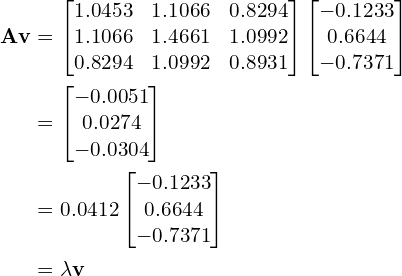
where
So, an Eigen vector ![]() of a matrix
of a matrix ![]() is a vector whose direction does not change when the matrix is multiplied to it. In other words,
is a vector whose direction does not change when the matrix is multiplied to it. In other words,
![]()
where
How to Calculate PCA?
Usually, you can easily find the principal components of given data using a linear algebra package of your choice. In the next post, we will learn how to use the PCA class in OpenCV. Here, we briefly explain the steps for calculating PCA so you get a sense of how it is implemented in various math packages.
Here are the steps for calculating PCA. We have explained the steps using 3D data for simplicity, but the same idea applies to any number of dimensions.
- Assemble a data matrix: The first step is to assemble all the data points into a matrix where each column is one data point. A data matrix,
 , of
, of  3D points would like something like this
- Calculate Mean: The next step is to calculate the mean (average) of all data points. Note, if the data is 3D, the mean is also a 3D point with x, y and z coordinates. Similarly, if the data is m dimensional, the mean will also be m dimensional. The mean
 is culculated as
- Subtract Mean from data matrix: We next create another matrix
 by subtracting the mean from every data point of

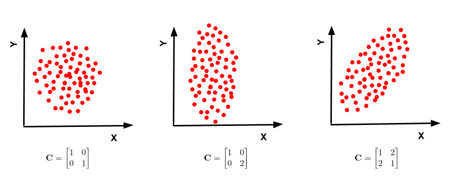
- Calculate the Covariance matrix: Remember we want to find the direction of maximum variance. The covariance matrix captures the information about the spread of the data. The diagonal elements of a covariance matrix are the variances along the X, Y and Z axes. The off-diagonal elements represent the covariance between two dimensions ( X and Y, Y and Z, Z and X ).The covariance matrix,
 is calculated using the following product.
where, represents the transpose operation. The matrix
  is of size
  where
where  is the number of dimensions ( which is 3 in our example ).Figure 5 shows how the covariance matrix changes depending on the spread of data in different directions.
If you are more interested in why this procedure works, here is an excellent article titled A Geometric Interpretation of the Covariance Matrix.
There is another widespread dimensionality reduction and visualization technique called t-SNE.



100K+ Learners
Join Free OpenCV Bootcamp3 Hours of Learning