Pix2Pix:Image-to-Image Translation in PyTorch & TensorFlow

Continuing our Generative Adversarial Network a.k.a. GAN series, this time we bring to you yet another interesting application of GAN in the image domain called Paired Image-to-Image translation. By now, you have seen many different types of GANs, all having a generator and discriminator that trained in unison. And in every GAN, the generator is fed a random-noise vector, while the discriminator is fed real or fake images that may or may not be conditioned on class labels.

But things are different in Paired Image-to-Image translation or Pix2Pix as it’s more commonly known. It deviates from the idea of feeding a random-noise vector to the generator and incorporates several significant architectural changes, though it does borrow a lot from the previous GAN algorithms.

In Image-to-Image Translation, the task is to translate images from one domain to another by learning a mapping between the input and output images, using a training dataset of aligned or unaligned cross-domain image pairs.

An image-to-image translation can be paired or unpaired. This post focuses on Paired Image-to-Image Translation. We will be covering Unpaired Image-to-Image Translation in detail in another post.

1. Paired Image-to-Image Translation
2. Applications of Pix2Pix
3. What is a Pix2Pix GAN?
4. UNET Generator
5. PatchGAN Discriminator
6. Pix2Pix Loss
7. Coding a Pix2Pix in PyTorch with Multi-GPU Training
8. Coding a Pix2Pix in TensorFlow with Multi-GPU Training
9. Results
10. Conclusion

Paired Image-to-Image Translation (Pix2Pix)

In paired image-to-image translation, the input and the ground-truth image domains are aligned. While paired training samples might be difficult to obtain, this type of translation often leads to great results. In the above image, we have various paired image-to-image translation tasks. For example:

• A segmentation map of an urban-scene is translated to an RGB image (street-scene) with all the contents of the input image preserved.
• There’s the  semantic segmentation (labels) to a street-scene task, which calls for paired training because you do not want to generate a completely random scene, given a label of a specific scenario. 
• In yet another translation task, the black and white image of a flower is translated to a colored image, with the flower and overall input image contents very much present in the translated color image.

This post is part of the series on Generative Adversarial Networks in PyTorch and TensorFlow, which consists of the following tutorials:

1. Introduction to Generative Adversarial Networks (GANs)
2. Deep Convolutional GAN in Pytorch and TensorFlow
3. Conditional GAN (cGAN) in PyTorch and TensorFlow
4. Pix2Pix: Paired Image-to-Image Translation in PyTorch and TensorFlow

Applications of Pix2Pix

• Transforming a black and white image to a colored image.
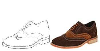
• Transforming edges into a meaningful image, as shown in the sandal image above, where given a boundary or information about the edges of an object, we realize a sandal image.
• Converting an aerial or satellite view to a map.
• Generating a segmentation map from a realistic image of an urban scene, comprising a road, sidewalk, pedestrians etc.
• Translating a photograph from day to a night time scenario or vice-versa. It has proved useful in downstream data augmentation.
• Transforming a low-resolution image to a high-resolution one, as shown in the video below.

Now, if you think carefully, all the above applications have one thing in common, i.e., we are doing a type of conditional generation, conditioned on the input image’s content. For example, in transforming the black and white image to color, the contents or the structure of the former black and white image on which this new image has been conditioned should be preserved.

What is a Pix2Pix GAN?

In 2016, a group of scholars led by Phillip Isola, at Berkeley AI Research (BAIR) published the paper titled Image-to-Image Translation with Conditional Adversarial Networks and later presented it at CVPR 2017. This paper has gathered more than 7400 citations so far!

Guess what inspired Pix2Pix. It was the Conditional GAN (CGAN), which again was an extension of the DCGAN architecture. So, if you haven’t read our previous GAN posts, we highly recommend you go through them once to understand this topic better. Some quick points to recap:

• Be it a vanilla GAN or DCGAN, the architecture as you will recall consisted  of two networks: the generator and the discriminator. Both trained in tandem, the generator tried to mimic the real data distribution, while the discriminator network learned to classify real from fake (generated). 
• After the training, the generator input random noise to output realistic images similar to the ones in the dataset.
• While the generator produced realistic-looking images, we certainly had no control over the type or class of generated images. Hence, came CGAN  allowing controlled generation. An extension of the GAN architecture, CGAN  generated images conditioned on class labels. 
  • The generator was fed a random-noise vector conditioned on class label.
  • And the discriminator was fed real or fake (generated) images conditioned on the class label.

Pix2Pix GAN further extends the idea of CGAN, where the images are translated from input to an output image, conditioned on the input image. Pix2Pix is a Conditional GAN that performs Paired Image-to-Image Translation.

The generator of every GAN we read till now was fed a random-noise vector, sampled from a uniform distribution. But the  Pix2Pix GAN eliminates the noise vector concept totally from the generator.

In Pix2Pix:

• An image is input to the generator network, which then outputs a translated version. 
• The discriminator is a conditional discriminator, which is fed a real or fake (generated) image that has been conditioned on the same input image that was fed to the generator. 
• The goal of the discriminator is to classify whether the pair of images is real (from the dataset) or fake (generated). 
• The final objective of the Pix2Pix GAN remains  the same as that of all the GANs. It too seeks to fool the discriminator, such that the generator learns to translate images perfectly.

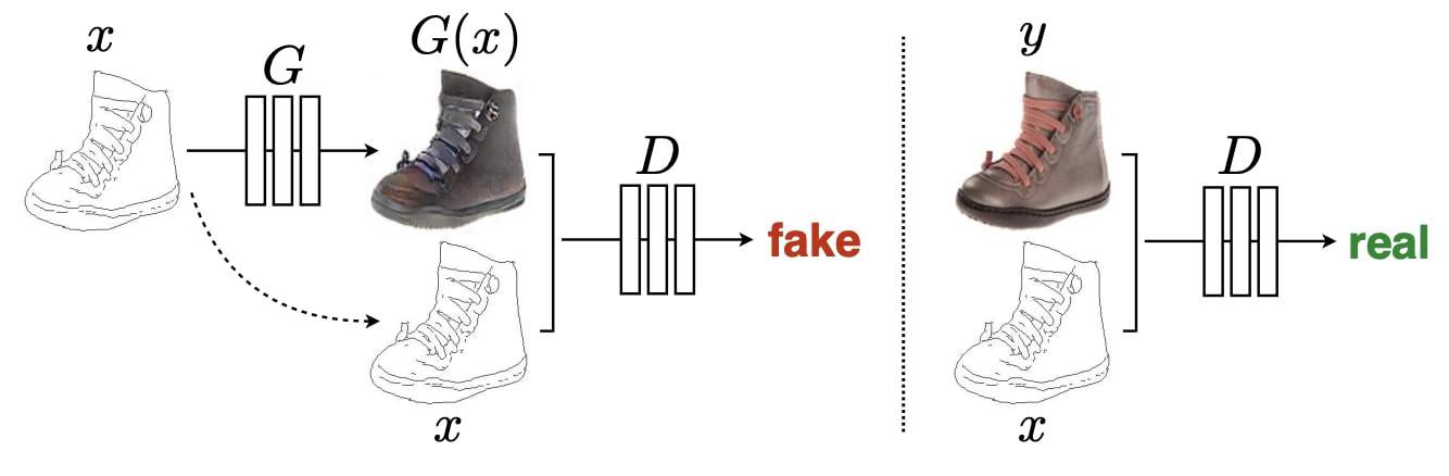
To develop better intuition, let’s refer to the above image in which a conditional GAN is trained to map edges->photo. Given an input edge image (before translation) , 

1. The generator learns to produce a translated shoe photo similar to the real shoe photo . 
2. The discriminator learns to classify 
   1. the generated photo , conditioned on input , as fake
   2.   the real photo , conditioned on input , as real. 
3. Unlike an uncontrolled GAN, both the generator and discriminator observe the input-edge map.

In earlier GAN architectures, the noise vector helped generate different outputs by adding randomness to it. But this was of not much use in Pix2Pix GAN, so the authors did away with it. They found a way though to keep the minor stochasticity in the output of the generator, i.e., by adding Dropout in the Generator Network (Consider heading to the Pix2Pix Implementation section to see how it works!).

UNET Generator

All the generator architectures you have seen so far input a random-noise vector (that may or may not be conditioned on a class label) to generate an image. So all these generator networks work like the Decoder of an Autoencoder, i.e., taking a latent-vector to output an image.

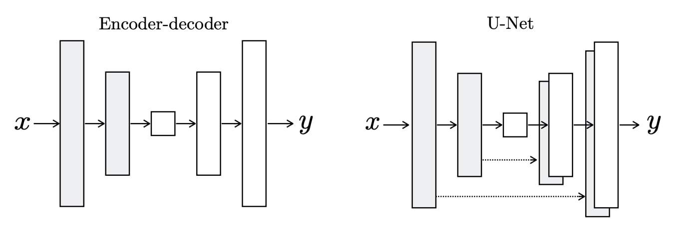
But the scene changes in Pix2Pix.  It rejects the traditional generator architecture to adopt the Autoencoder style, which has both Encoder and Decoder networks. But why? The answer is pretty straightforward. In Pix2Pix, unlike traditional GAN architectures, both input and output is an image. And what’s better than using an Autoencoder for this purpose.

What you find in Pix2Pix is a UNET Generator, comprising an Encoder-Decoder, with skip connections between the mirrored layers, in both the stacks.

The UNET Generator’s 

• Input could be edges, semantic-segmentation labels, black and white images etc.
• The output could be a photo (bag, shoe), street scene, colored image etc.

In an Autoencoder, the output is as close as possible to the input . But in a UNET Generator:

• This is a translated and conditioned version of . 
•  Also, skip-connections are introduced, which help recover all information lost during the downsampling of the input at Encoder. During backpropagation, it even helps improve the gradient flow by avoiding the vanishing gradient issue.

Pix2Pix PatchGAN Discriminator

The Pix2Pix Discriminator has the same goal as any other GAN discriminator, i.e., to classify an input as real (sampled from the dataset) or fake (produced by generator). Its architecture differs a bit though, mainly in terms of how the input is regressed at the output (final) layer.

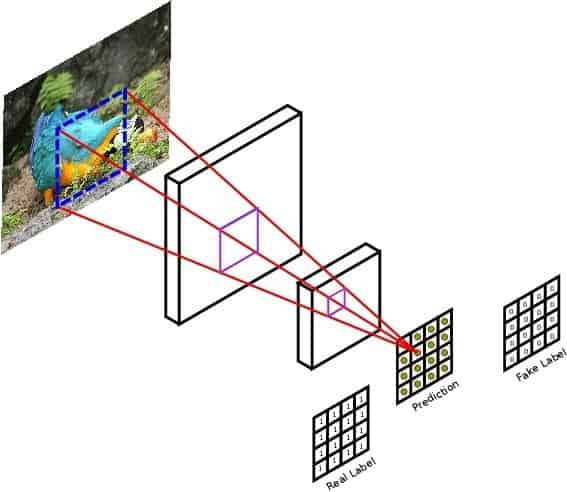
Called a PatchGAN, the Pix2Pix Discriminator outputs a tensor of values (30×30) instead of a scalar value in the range [0, 1], as seen in previous GAN architectures. Why the name PatchGAN but? Mainly because of the matrix of values that the discriminator outputs for a given input. Unlike the traditional GAN model that uses a CNN with a single output to classify images, the Pix2Pix model uses a thoughtfully-designed PatchGAN to classify patches (70×70) of an input image as real or fake, rather than considering the entire image at one go.

Some PatchGAN facts:

• The discriminator network uses standard Convolution-BatchNormalization-ReLU blocks of layers, as is common for deep-convolutional neural networks. 
• But the number of layers is configured such that the effective receptive field of each output of the network maps to a specific size in the input image. 
• The network outputs a single feature map of real/fake predictions that can be averaged to give a single score (loss value). More on this,when we implement  Pix2Pix.

Two main highlights of PatchGAN Discriminator are:

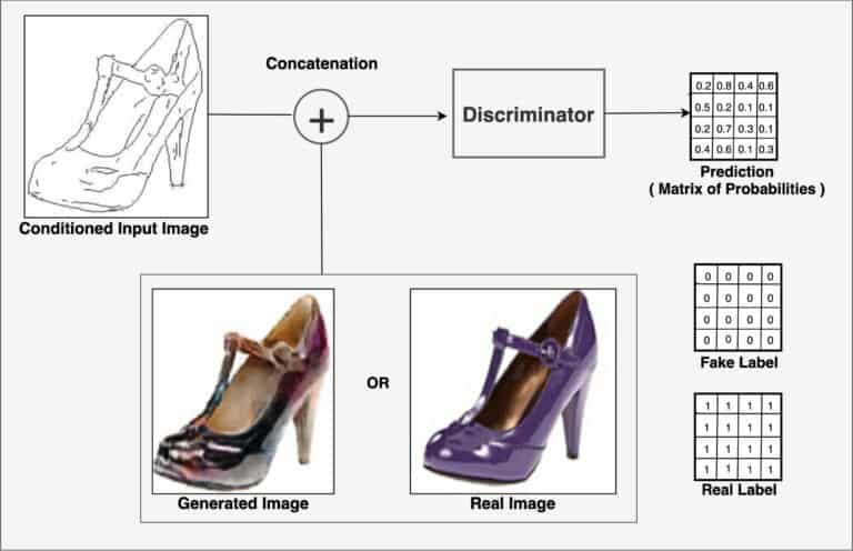
• Conditional Discriminator: Inspired by Conditional GAN, the discriminator is fed real or fake images conditioned on the input image. Hence, the input is a concatenated version of the real or fake image and the input image (edges, in case of edges->photos). With this condition, the discriminator tries to figure out whether the Real or Generated image actually looks like a realistic mapping of the input edge image or not.
• Patch: The input image of [256, 256, n_channels] dimension is classified in patches, meaning the output is a tensor of [30, 30] dimension, and not a scalar value. At the output, 
  • each [1, 1] in the [30, 30] tensor represents a patch of [70, 70] in the input image
  • each grid in this tensor of values is classified in the range [0, 1] , where 0 is fake, and 1 is real, as before. 

In the above image:

•  Each value of the output prediction matrix represents the probability of the corresponding image patch being real or fake (generated). 
• A patch size of 70×70 was found to be effective across a range of image-to-image translation tasks.

Excerpt from the paper:

We design a discriminator architecture – which we term a PatchGAN – that only penalizes structure at the scale of patches. This discriminator tries to classify if each NxN patch in an image is real or fake. We run this discriminator convolutionally across the image, averaging all responses to provide the ultimate output of D.

Advantages of the PatchGAN giving feedback on each local region or patch of the image:

1. The  discriminator can better classify real and fake images. 
2. It also helps the generator fool the discriminator, by generating even more realistic images. 

As it outputs the probability of each patch being real or fake, PatchGAN can be trained with the GAN loss i.e., the Binary Cross-Entropy (BCE) loss. 

Referring to the above image, let’s see how the PatchGAN output tensor changes for different images. 

• For a fake image from the generator, the PatchGAN will learn to output a tensor of all zeros, and the label for it would also be a matrix of all zeros. This means that the discriminator must output zeros for all the values in the matrix to achieve minimal loss. 
• For a real image, the PatchGAN will learn to output a tensor of all ones, and the label for it would be a matrix of all ones.

Pix2Pix Loss

To optimize both generator and discriminator, the standard training approach is followed i.e. alternate one gradient descent step on the Discriminator, with one on the Generator.

The following excerpt from the paper gives the crux of the Pix2Pix Loss:

The discriminator’s job remains unchanged, but the generator is tasked to not only fool the discriminator but also to be near the ground-truth output in an L2 sense. We also explore this option, using L1 distance rather than L2 as L1 encourages less blurring.

Discriminator

The Pix2Pix discriminator network is trained with the same loss as the previous GANs like the DCGAN, CGAN etc. i.e., the Adversarial Loss (Binary Cross-Entropy (BCE)). The discriminator’s objective here is to minimize the likelihood of a negative log identifying real and fake images.

To slow down the rate at which the discriminator learns relative to the generator, the authors divided the loss by 2 at the time of the optimization of the discriminator.

The total discriminator loss is given as:

(1)  

Generator

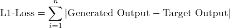
Real labels are used to train the generator network with the adversarial loss (BCE Loss) for generated images. It also has an additional loss, i.e., an L1 loss, which is used to minimize the error. 

• This additional loss is the sum of all the absolute differences between the true value and the predicted value. 
• L1 loss acts as a regularization term, penalizing the generator if the reconstruction quality of the translated image is not similar to the target image.

In the generator’s context, the L1 loss is the sum of all the absolute pixel differences between the generator output (translated version of the input image) and the real target (ground-truth/expected target image).

(2)  

The total generator loss is given as:

(3)  

The combined loss is governed by a hyperparameter , where is used to weigh the second term. The authors did an ablation study and found better suited the BCE loss for it reduced the artifacts, and at the same time, produced sharper images. They evaluated L2 loss too, but found it produced blurry images.

This much theory will do, let’s move on to the coding now and get set to implement Pix2Pix, both in TensorFlow and PyTorch, with Multi-GPU.

Coding a Pix2Pix in PyTorch with Multi-GPU

Pix2Pix Dataset

We use the Edges→Shoes dataset, which has 50K shoes, originally collected from Zappos.com.

This dataset contains:

• 50k training images from UT Zappos50K dataset. The shoes (shown on the right) are roughly centered, but not well aligned. They face a little to the left, offering a frontal to the side view.
• The input images (as shown on the right) are binary edges generated with the Holistically-Nested Edge Detector (HED).
• Each image is of size 256 x 256 pixels, with three channels, i.e., an RGB image.
• Random jitter and Random Mirroring was applied, by resizing the 256×256 input images to 286 × 286, and then randomly cropping them back to size 256 × 256.
• You can download the dataset from here.

Note: All the implementations were carried out on a DGX V100 GPU.

Data Loading and Preprocessing

We have hardly seen any preprocessing, apart from resizing and normalizing the image, in any of our previous GAN posts.

However, in Pix2Pix, the authors did employ a couple of preprocessing and augmentation techniques like random jittering and random mirroring. So let’s see how we can implement them in PyTorch.

'''Data Preprocessing'''
    
def read_image(image):
        
        image = np.array(image)
        width = image.shape[1]
        width_half = width // 2
       
        input_image = image[:, :width_half, :]
        target_image = image[:, width_half:, :]
    
        input_image = input_image.astype(np.float32)
        target_image = target_image.astype(np.float32)
    
        return input_image, target_image

Click here to download the source code to this post

• The read_image function is fed images from the PyTorch dataloader. The dataloader uses a pillow package that reads images as an object. So, we first convert it to a NumPy array.

• The dataset, as shown in the above image, has both the input and ground-truth images concatenated along the width dimension. We separate them in the image reading function. 
• After the image is read, basic Numpy slicing and indexing is done to create input_image and target_image (Line 9-10).

  def random_crop(image, dim):
    height, width, _ = dim
    x, y = np.random.uniform(low=0,high=int(height-256)), np.random.uniform(low=0,high=int(width-256))  
    return image[:, int(x):int(x)+256, int(y):int(y)+256]

    

def random_jittering_mirroring(input_image, target_image, height=286, width=286):
    
    #resizing to 286x286
    input_image = cv2.resize(input_image, (height, width) ,interpolation=cv2.INTER_NEAREST)
    target_image = cv2.resize(target_image, (height, width),
                               interpolation=cv2.INTER_NEAREST)
    
    #cropping (random jittering) to 256x256
    stacked_image = np.stack([input_image, target_image], axis=0)
    cropped_image = random_crop(stacked_image, dim=[IMG_HEIGHT, IMG_WIDTH, 3])
    
    input_image, target_image = cropped_image[0], cropped_image[1]
    #print(input_image.shape)
    if torch.rand(()) > 0.5:
     # random mirroring
        input_image = np.fliplr(input_image)
        target_image = np.fliplr(target_image)
    return input_image, target_image

• Next, we perform random_jittering and random_mirroring.

For random jittering:

• Resize both the images from 256×256 to 286×286, using the opencv resize method, with nearest-neigbour interpolation.
• Then stack both images along the 1st dimension, using Numpy’s stack method. This returns an array with dimension [2, 286, 286, 3]. Stack both the images because in the next step, when we do a random crop operation,  we want both the images cropped alike.
• Finally, the stacked image is fed to the random_crop function, which randomly samples and coordinates from a uniform distribution, in the range [0, resize_dim – crop_dim]. We then get a crop of 256×256, by  Numpy slicing and indexing the stacked image, based on the new and coordinates added to the required crop size.

The random mirroring is quite straightforward:

• To randomize the process, sample a point from a uniform distribution in the interval [0, 1].
• If the point sampled is greater than 0.5, both the input and target image are flipped left-right.

def normalize(inp, tar):
    input_image = (inp / 127.5) - 1
    target_image = (tar / 127.5) - 1
    return input_image, target_image

• Next comes simple normalization of the input and target images. Both are normalized in a range [-1, 1], by dividing the image with 127.5 , and subtracting by 1.

class Train(object):
    def __call__(self, image):
        inp, tar = read_image(image)
        inp, tar = random_jittering_mirroring(inp, tar)
        inp, tar = normalize(inp, tar)
        image_a = torch.from_numpy(inp.copy().transpose((2,0,1)))
        image_b = torch.from_numpy(tar.copy().transpose((2,0,1)))
        return image_a, image_b

• Now define the Train class, which will be passed to the PyTorch transforms-compose method. Instead of using PyTorch’s built-in transform methods, we created our own transform methods. In the above function, we basically call the read_image, random_jittering_mirroring and normalize functions.
• In Line 50-51, we first change the channel dimensions from channel_last to channel_first , in line with the expectations of the  PyTorch model. Then convert the NumPy array to a Torch tensor.

DIR = 'edges2shoes/train_data/'
n_gpus = 4
batch_size = 64
global_batch_size = batch_size * n_gpus

train_ds = ImageFolder(DIR, transform=transforms.Compose([
        Train()]))
train_dl = DataLoader(train_ds, global_batch_size)

• Finally, define the training data directory, batch_size, and the number of GPUs we would be training our model on (Multi-GPU). Note: The global_batch_size is equal to the batch size multiplied by the total number of GPUs. This means:
  •  Each forward pass and backward pass will have a total of 512 (64 x 4) images
  • Each of the four GPUs will have 64 images.
• We pass the training directory and preprocessing transform function to the ImageFolder, which is further fed to the DataLoader , along with global batch size.

Now that our training data pipeline is ready, let’s move on to creating the generator and discriminator network architecture of Pix2Pix.

Pix2Pix Generator and Discriminator Architecture

In the theoretical section, you learned that the Generator used in Pix2Pix is an Encoder-Decoder with skip-connections, while the Discriminator is a fully-convolutional patch-based Binary Classifier. It’s time to implement both in PyTorch.

# custom weights initialization called on generator and discriminator
def init_weights(net, init_type='normal', scaling=0.02):
    def init_func(m):  # define the initialization function
        classname = m.__class__.__name__
        if hasattr(m, 'weight') and (classname.find('Conv')) != -1:
            torch.nn.init.normal_(m.weight.data, 0.0, scaling)
        elif classname.find('BatchNorm2d') != -1:  # BatchNorm Layer's weight is not a matrix; only normal distribution applies.
            torch.nn.init.normal_(m.weight.data, 1.0, scaling)
            torch.nn.init.constant_(m.bias.data, 0.0)

    print('initialize network with %s' % init_type)
    net.apply(init_func)  # apply the initialization function <init_func>

The init_weights function:

• Initializes the weights and biases of both the Convolution and BatchNorm layers used in the Generator and Discriminator network.
• The weights are initialized from a Gaussian/Normal distribution, with mean 0 and standard deviation 0.02. 
• It iterates layer by layer over the model, checks if the layer is Conv or BatchNorm2d, and initializes them accordingly.

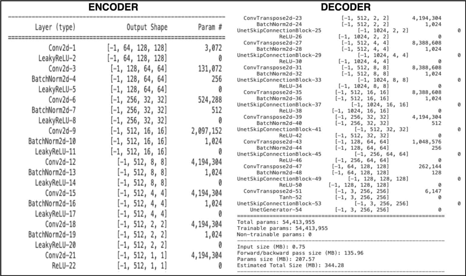
U-NET Generator

class UnetGenerator(nn.Module):
    """Create a Unet-based generator"""

    def __init__(self, input_nc, output_nc, nf=64, norm_layer=nn.BatchNorm2d, use_dropout=False):
        super(UnetGenerator, self).__init__()
        # construct unet structure
        # add the innermost block
        unet_block = UnetSkipConnectionBlock(nf * 8, nf * 8, input_nc=None, submodule=None, norm_layer=norm_layer, innermost=True) 
        #print(unet_block)

        # add intermediate block with nf * 8 filters
        unet_block = UnetSkipConnectionBlock(nf * 8, nf * 8, input_nc=None, submodule=unet_block, norm_layer=norm_layer, use_dropout=use_dropout)
        unet_block = UnetSkipConnectionBlock(nf * 8, nf * 8, input_nc=None, submodule=unet_block, norm_layer=norm_layer, use_dropout=use_dropout)
        unet_block = UnetSkipConnectionBlock(nf * 8, nf * 8, input_nc=None, submodule=unet_block, norm_layer=norm_layer, use_dropout=use_dropout)

        # gradually reduce the number of filters from nf * 8 to nf. 
        unet_block = UnetSkipConnectionBlock(nf * 4, nf * 8, input_nc=None, submodule=unet_block, norm_layer=norm_layer)
        unet_block = UnetSkipConnectionBlock(nf * 2, nf * 4, input_nc=None, submodule=unet_block, norm_layer=norm_layer)
        unet_block = UnetSkipConnectionBlock(nf, nf * 2, input_nc=None, submodule=unet_block, norm_layer=norm_layer)
        
        # add the outermost block
        self.model = UnetSkipConnectionBlock(output_nc, nf, input_nc=input_nc, submodule=unet_block, outermost=True, norm_layer=norm_layer)  

    def forward(self, input):
        """Standard forward"""
        return self.model(input)

Constructing the U-NET 

The U-NET Generator’s implementation is divided into three parts: outermost, innermost and intermediate blocks. We construct the U-Net from the innermost layer to the outermost layer in a recursive fashion. The class UnetGenerator constructor takes the following parameters:

1. input_nc (int) — the number of channels in input images/features
2. output_nc (int) — the number of channels in output images/features
3. nf (int) — the number of filters in the first conv layer
4. norm_layer — normalization layer
5. takes the above  parameters. Apart from these, it also takes a fifth parameter called submodule , which is nothing but the output from the previous block. 

The class has a special function called UnetSkipConnectionBlock to do this job.

It’s important to note that on an abstract level:

• Each unet_block comprises a block (Conv2D/ConvTranspose2d + BatchNorm + Activation) of both Encoder and Decoder. 
• Also, there are no max-pooling layers
•  Strided convolutions are used, with a stride of 2
•  Each Conv layer downsamples the image by a factor of 2.

Starting with the Outermost Block

In Line 94, we define the outermost block, i.e., the first and last layer of the generator. The outermost block is fed:

•  output_nc=3
•  nf=64
•  input_nc=3, with submodule=unet_block and outermost=True (this flag tells the class UnetSkipConnectionBlock to execute only those statements that satisfy the ‘outermost’ flag)

The submodule parameter fits the preceding block within the current block. The outermost block thus will be fed a submodule block, which lies between the first and last layer of the model. For example, assume we have a four-layer neural network. Now, the outermost block will have the first and fourth layers, while the intermediate block (submodule) will have the second and third layers, sandwiched between the two layers of the outermost block. To make things crystal clear, have a look at the image below. Assume ‘None’ is a submodule that represents the layers fitted within the outermost block.

Let’s unroll the outermost layer and see what is in it. To achieve this, comment out the other blocks, and give the submodule parameter as None:

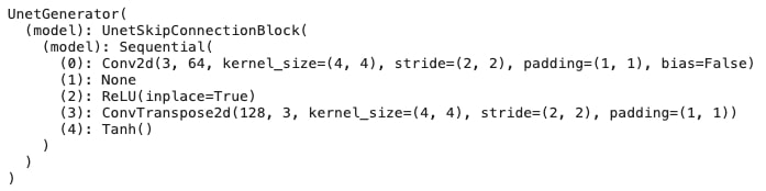
Well, as you can see in the above image: 

1. The first layer is a Conv2d layer, with input_nc=3 (input to the model is an RGB image). 
2. Followed by a None. The reason is quite simple, we gave the submodule parameter as None. 
3. Finally, we have a block (ReLU + ConvTranpose2d + Tanh), which is the last block of the Generator. Dig deeper, you’ll see the ConvTranspose2d has input_nc=128 and output_nc=3, meaning that this layer expects 128 channels from the preceding block. Also that it will produce a 3-channel result. And isn’t that exactly what we need —an image with 3 channels at the end. Right? 

The Intermediate and Innermost Blocks

Similarly, we have the intermediate blocks (Lines 89 – 91), which increase the number of filters (feature maps) from nf to nf * 8 in the Encoder, and vice-versa in the Decoder. Isn’t that what generally happens in an Autoencoder, right? We feed an image to the Encoder, compress the spatial dimensions, while increasing the feature maps as we reach the bottleneck. Then perform the exact opposite in the decoder to produce an image at the output. So the intermediate blocks do the job of the Autoencoder in the UnetGenerator.

We have a second set of intermediate blocks (Lines 84 – 86), having nf=512, in all three blocks. While the number of filters remains constant, the image is downsampled by a factor of 2, i.e., from 8×8->4×4->2×2, and vice-versa (remember, each block does downsampling as well as upsampling, putting submodules in between). Finally, the innermost block (Line 80) further downsamples (2×2->1×1) and upsamples the image. The innermost block is basically the bottleneck of the UnetGenerator. Note that the submodule parameter is None because no way can we put another layer in what we told you is the bottleneck block.

class UnetSkipConnectionBlock(nn.Module):
    def __init__(self, outer_nc, inner_nc, input_nc=None,
                 submodule=None, outermost=False, innermost=False, norm_layer=nn.BatchNorm2d, use_dropout=False):
        super(UnetSkipConnectionBlock, self).__init__()
        self.outermost = outermost
        if input_nc is None:
            input_nc = outer_nc
        downconv = nn.Conv2d(input_nc, inner_nc, kernel_size=4,
                             stride=2, padding=1, bias=False)
        downrelu = nn.LeakyReLU(0.2, True)
        downnorm = norm_layer(inner_nc)
        uprelu = nn.ReLU(True)
        upnorm = norm_layer(outer_nc)

        if outermost:
            upconv = nn.ConvTranspose2d(inner_nc * 2, outer_nc,
                                        kernel_size=4, stride=2,
                                        padding=1)
            down = [downconv]
            up = [uprelu, upconv, nn.Tanh()]
            model = down + [submodule] + up
        elif innermost:
            upconv = nn.ConvTranspose2d(inner_nc, outer_nc,
                                        kernel_size=4, stride=2,
                                        padding=1, bias=False)
            down = [downrelu, downconv]
            up = [uprelu, upconv, upnorm]
            model = down + up
        else:
            upconv = nn.ConvTranspose2d(inner_nc * 2, outer_nc,
                                        kernel_size=4, stride=2,
                                        padding=1, bias=False)
            down = [downrelu, downconv, downnorm]
            up = [uprelu, upconv, upnorm]

            if use_dropout:
                model = down + [submodule] + up + [nn.Dropout(0.5)]
            else:
                model = down + [submodule] + up

        self.model = nn.Sequential(*model)

    def forward(self, x):
        if self.outermost:
            return self.model(x)
        else:   # add skip connections
            return torch.cat([x, self.model(x)], 1)

It’s in the UnetGenerator class, which you have now understood in great detail, along with the working of UnetSkipConnectionBlock,  that we write all the three blocks. The trio then combines to form a Unet-based Generator.

Lines 106-109 form an Encoder (Strided Conv + LeakyRelu + Batchnorm), which are part of all three blocks: outer, inner and intermediate.

Lines 110-111 are fed to the Generator’s Decoder part, i.e., uprelu and upnorm. Note how the innermost condition has no submodule, just the Encoder (down) and Decoder (up) part for it forms the network’s bottleneck part.

The outermost condition, as discussed earlier, corresponds to the first and last layers of the network. 

• The up part follows a Tanh activation function at the end, as our dataset images are normalized in the range [-1, 1].
• Both the Conv2d and ConvTranspose2d layers use a filter size 4, stride 2, padding 1, and bias is set to False. 
• The Encoder uses LeakyReLU activation, with a slope of 0.2, along with the batchnorm layer. 
• The Decoder however prefers to go for ReLU activation with the batchnorm layer.

One last and important part is adding the skip-connection, which happens on Line 145. Note that the skip-connections do not apply in the outermost block (first and the last layer): 

• The first layer will have no information from the preceding layer
• While the final layer will be a three-channel image requiring no concatenation. 

That’s how a UNET is structured.

How does the concatenation happen? Assume the innermost block receives x from the preceding layer, having [batch, 512, 2, 2] dimensions, when we call self.model(x) ( Line 145 ):

• The input is first fed to a series of Encoder layers: strided conv layer + activation + norm, producing an output of [batch, 512, 1, 1].
• The output produced above then goes through Decoder layers: strided convtranspose layer + activation + norm, producing an output of [batch, 512, 2, 2].

These two steps make one self.model(x) call, and now you can see that the input x from the preceding layer along with self.model(x) produces a result that can be concatenated. And that’s how skip-connections are implemented here.

Enabling Multi-GPU

device = torch.device('cuda' if torch.cuda.is_available() else 'cpu')
print(torch.cuda.device_count())
generator = UnetGenerator(3, 3, 64, norm_layer=norm_layer, use_dropout=False).cuda().float()
init_weights(generator, 'normal', scaling=0.02)
generator = torch.nn.DataParallel(generator)  # multi-GPUs

Enabling multi-GPU in PyTorch is quite simple. 

• First check if PyTorch is using the cuda
• Then do a sanity check on the device count (GPU count).
• Next,  move the Generator on the GPU, by calling .cuda(), which anyways is required even when you train with a single GPU.
• In Line 5, the magic of multi-GPU takes place, by passing the generator model as a parameter to the DataParallel module.

What is a DataParallel Module?

The DataParallel module parallelizes the model by splitting the input across the specified devices, and chunking in the batch dimension (other objects will be copied once per device). 

• In the forward pass, the module is replicated on each device, and each replica handles a portion of the input. 
• During the backward pass, gradients from each replica are summed into the original module. 

The global batch size should be larger than the number of GPUs used. You can also pass the device ids to the Dataparallel module, which conditions the data to be split on the specified device ids. This sure is handy when you have 8-16 GPUs but want to run your model on not more than 2-5 GPU ids.

PatchGAN Discriminator

The discriminator is a patch-based binary classifier that is fed a real or fake (generated) image. As we know, its goal is to classify the given image as real or fake, but in Pix2Pix, we predict at a patch level (30×30) rather than outputting a scalar number. You have already covered all this here so let’s not go into details again.

class Discriminator(nn.Module):
    def __init__(self, input_nc, ndf=64, n_layers=3, norm_layer=nn.BatchNorm2d):
        super(Discriminator, self).__init__()
        kw = 4
        padw = 1
        sequence = [nn.Conv2d(input_nc, ndf, kernel_size=kw, stride=2, padding=padw), nn.LeakyReLU(0.2, True)]
        nf_mult = 1
        nf_mult_prev = 1
        for n in range(1, n_layers):  # gradually increase the number of filters
            nf_mult_prev = nf_mult
            nf_mult = min(2 ** n, 8)
            sequence += [
                nn.Conv2d(ndf * nf_mult_prev, ndf * nf_mult, kernel_size=kw, stride=2, padding=padw, bias=False),
                norm_layer(ndf * nf_mult),
                nn.LeakyReLU(0.2, True)
            ]

        nf_mult_prev = nf_mult
        nf_mult = min(2 ** n_layers, 8)
        sequence += [
            nn.Conv2d(ndf * nf_mult_prev, ndf * nf_mult, kernel_size=kw, stride=1, padding=padw, bias=False),
            norm_layer(ndf * nf_mult),
            nn.LeakyReLU(0.2, True)
        ]

        sequence += [nn.Conv2d(ndf * nf_mult, 1, kernel_size=kw, stride=1, padding=padw), nn.Sigmoid()]  # output 1 channel prediction map
        self.model = nn.Sequential(*sequence)

    def forward(self, input):
        """Standard forward."""
        return self.model(input)

The PatchGAN discriminator’s architecture is very straightforward but unlike any other GAN discriminator classifier. 

• All the convolution layers use a kernel size of 4, with a padding of 1
• Followed mostly by a LeakyReLU and the batchnorm layer
• The one, exception being the last layer, which has a sigmoid activation to get a probabilistic value in the range [0, 1].

At Line 156, you have the first strided convolution layer, which downsamples the image by a factor of 2, and expects an input_nc=6 (Remember, we condition discriminator by concatenating the shoe image with its paired-edge image), with 64 filters, followed by a LeakyReLU activation.

• We further downsample the image with a couple of strided convolution layers, doubling the filters at each layer, followed by LeakyReLU and batchnorm.
• By now, we have an output of dimension [batch, 256, 32, 32], but don’t forget we need an output of size 30×30. 
• You cannot afford to use another convolution layer with a stride of two. Hence, use a couple more convolution layers with a stride of one, thereby slowly reducing the spatial dimensions from 32->31->30, with just 1 filter at the last layer. 
• Finally, apply a sigmoid activation at the end. 

Just a reminder that each (1×1) of the 30×30 represents a 70×70 dimension in the input image (256×256), classifying a single patch of the original image as real or fake.

Loss Function

adversarial_loss = nn.BCELoss() 
l1_loss = nn.L1Loss()

The Binary Cross-Entropy loss is defined to model the objectives of the Generator and Discriminator networks. And a second reconstruction loss L1Loss is used for the generator.

Generator Loss

def generator_loss(generated_image, target_img, G, real_target):
    gen_loss = adversarial_loss(G, real_target)
    l1_l = l1_loss(generated_image, target_img)
    gen_total_loss = gen_loss + (100 * l1_l)
    #print(gen_loss)
    return gen_total_loss

Four parameters are fed to the generator_loss function:

• generated_image: Images produced by the generator
• target_image: Ground-truth pair image for the input fed to the generator.
• G: Output predictions from the discriminator, when fed with generator-produced images.
• real_target: Ground-truth labels (1), as you would like the generator to produce real images by fooling the discriminator. The labels therefore would be one.

The adversarial loss is fed prediction G and real_target labels, while the l1_loss computes the reconstruction error between the generated and target image.

Multiply by 100 to weigh the l1_loss. The final loss is the sum of both losses.

Discriminator Loss

def discriminator_loss(output, label):
    disc_loss = adversarial_loss(output, label)
    return disc_loss

The discriminator loss has

• the real (original images) output predictions ground-truth label as 1
• Fake (generated images) output predictions ground-truth label as 0. 

The discriminator loss will be called twice during the training, on the same batch of images: once for real images and once for the fakes.

Training the Pix2Pix

num_epochs = 200
D_loss_plot, G_loss_plot = [], []
for epoch in range(1, num_epochs+1): 
  

    D_loss_list, G_loss_list = [], []
   
    for (input_img, target_img), _ in train_dl:
       
        D_optimizer.zero_grad()
        input_img = input_img.to(device)
        target_img = target_img.to(device)

        # ground truth labels real and fake
        real_target = Variable(torch.ones(input_img.size(0), 1, 30, 30).to(device))
        fake_target = Variable(torch.zeros(input_img.size(0), 1, 30, 30).to(device))
        
        # generator forward pass
        generated_image = generator(input_img)
        
        # train discriminator with fake/generated images
        disc_inp_fake = torch.cat((input_img, generated_image), 1)
        
        D_fake = discriminator(disc_inp_fake.detach())
        
        D_fake_loss   =  discriminator_loss(D_fake, fake_target)
        
        # train discriminator with real images
        disc_inp_real = torch.cat((input_img, target_img), 1)
                                
        D_real = discriminator(disc_inp_real)
        D_real_loss = discriminator_loss(D_real,  real_target)

    
        
        # average discriminator loss
        D_total_loss = (D_real_loss + D_fake_loss) / 2
        D_loss_list.append(D_total_loss)
        # compute gradients and run optimizer step
        D_total_loss.backward()
        D_optimizer.step()
        
        
        # Train generator with real labels
        G_optimizer.zero_grad()
        fake_gen = torch.cat((input_img, generated_image), 1)
        G = discriminator(fake_gen)
        G_loss = generator_loss(generated_image, target_img, G, real_target)                                 
        G_loss_list.append(G_loss)
        # compute gradients and run optimizer step
        G_loss.backward()
        G_optimizer.step()

The training of Pix2Pix is quite similar to the GANs we have covered so far. However, there are few modifications:

1. The ground-truth labels (Line 207-208): Real and fake targets have a dimension of [batch, 1, 30, 30], as Pix2Pix uses a Patch-based Discriminator, where the input image is regressed to a patch of 30×30 dimension.
2. The discriminator of Pix2Pix you know is conditioned on the input image, so before feeding the real image or the generated image to the discriminator, concatenate the input image along the channel dimension (Line 214, 221 & 238).

That’s all you need to modify in the training part, and voila, your Pix2Pix network learns to create realistic shoe images from the shoe drawings (or edges).

Results

While training Pix2Pix, we also monitor the progress of our network through qualitative results. So we prepare a separate validation dataloader, with 200 images in the data loading and preprocessing step, only this time there is no random jittering or mirroring.

for (inputs, targets), _ in val_dl:
    inputs = inputs.to(device)
    generated_output =  generator(inputs)
    save_images(generated_output.data[:10], 'sample_%d'%epoch + '.png', nrow=5, normalize=True)

After each epoch, we iterate over the validation data, infer with the generator, and save 10 images. And the results are below for you to see.

Looks like our Generator did a decent job for it generated various types of footwear like sandal, sneaker, boots etc. But yes,  there definitely is room for improvement. Play around with the code and see if you can improve the quality of images even more.

Done with training and validation, let’s now move on to implement the Pix2Pix in TensorFlow.

Coding a Pix2Pix in TensorFlow with Multi-GPU

We will implement the Pix2Pix in the TensorFlow framework, on the same Edges→Shoes dataset that we used in the PyTorch implementation.

Data Loading and Preprocessing

Data loading and preprocessing in TensorFlow is almost identical to Pytorch. So,  if you followed the Pytorch implementation well, this will be a cakewalk.

def read_image(image_path):
    image = tf.io.read_file(image_path)
    image = tf.image.decode_image(image, channels=3)
    
    width = tf.shape(image)[1]
    width_half = width // 2
    
    input_image = image[:, :width_half, :]
    target_image = image[:, width_half:, :]
    
    input_image = tf.cast(input_image, dtype=tf.float32)
    target_image = tf.cast(target_image, dtype=tf.float32)
    return input_image, target_image

• We define the image reading function, which reads the image paths and decodes the images. The decode image function detects whether an image is a BMP, GIF, JPEG or PNG, and accordingly converts the input bytes string (read_file) into a Tensor of type dtype. 
• We also pass an additional input channels = 3 , which tells TensorFlow that the number of color channels is three (defaults to 0).

In the dataset, both the input and ground-truth images are concatenated widthwise, as shown in the above image. 

• We separate them in the image-reading function. 
• After the image is read, we find the shape of the tensor, extract the width, divide it by two and slice and index the tensor image to create input_image and target_image (Line 8-9).

@tf.function
def random_jittering_mirroring(input_image, target_image, height=286, width=286):
    
    #resizing to 286x286
    input_image = tf.image.resize(input_image, [height, width],method=tf.image.ResizeMethod.NEAREST_NEIGHBOR)

    target_image = tf.image.resize(target_image, [height, width],method=tf.image.ResizeMethod.NEAREST_NEIGHBOR)

                                   
    #cropping (random jittering) to 256x256
    stacked_image = tf.stack([input_image, target_image], axis=0)
    cropped_image = tf.image.random_crop(stacked_image, size=[2, IMG_HEIGHT, IMG_WIDTH, 3])
    
    input_image, target_image = cropped_image[0], cropped_image[1]
    
    if tf.random.uniform(()) > 0.5:
    # random mirroring
        input_image = tf.image.flip_left_right(input_image)
        target_image = tf.image.flip_left_right(target_image)
        
        
    return input_image, target_image

• Next, we perform random_jittering and random_mirroring. Unlike PyTorch, where we did the augmentations with the help of Numpy,  TensorFlow has its own built-in functions just for this.

To do random jittering we:

• Resize both the images from 256×256 to 286×286, using tf.image.resize method, with nearest-neigbour interpolation method.
• Then stack both the images along the 1st dimension, using tf.stack method. This returns an array, with dimension [2, 286, 286, 3]. We stack both images because in the next step we will perform a random crop operation, and both images should be cropped alike.
• Finally, the stacked image is fed to the tf.image.random_crop function, which will randomly crop a patch of size [2, 256,256,3]. As this patch will have two images: input image and target image, index the cropped image to get both .

Random mirroring is quite straightforward:

• To randomize the process, sample a point from a uniform distribution in the interval [0, 1].
• If the point sampled is greater than 0.5, both input and target images are flipped left-right, using tf.image.flip_left_right.

def normalize(input_image, target_image):
    input_image = (input_image / 127.5) - 1
    target_image = (target_image / 127.5) - 1
    return input_image, target_image

Then follows a simple normalization operation of the input and target images. Both are normalized in a range [-1, 1], by dividing the image with 127.5 , and subtracting by 1.

def preprocess_fn(image_path):
    input_image, target_image = read_image(image_path)
    input_image, target_image = random_jittering_mirroring(input_image, target_image)
    input_image, target_image = normalize(input_image, target_image)
    return input_image, target_image    

The above preprocess function calls the functions (read_image, normalize etc.) we defined above. These will be fed to the train dataloader that we will create in our next step.

image_paths = glob.glob('edges2shoes/train/*')

AUTOTUNE = tf.data.experimental.AUTOTUNE
mirrored_strategy = tf.distribute.MirroredStrategy()

n_gpu = 4
batch_size = 64
global_batch_size = batch_size * n_gpu

train_dataset = tf.data.Dataset.from_tensor_slices(image_paths)
train_dataset = train_dataset.map(preprocess_fn,
           num_parallel_calls=AUTOTUNE)                                  
train_dataset = train_dataset.shuffle(BUFFER_SIZE)
train_dataset = train_dataset.batch(global_batch_size)

train_dataset = mirrored_strategy.experimental_distribute_dataset(train_dataset)

In Line 46, 

• We use glob to fetch and list all the training images. 
• Then define AUTOTUNE, which increases the training time, by fetching and loading the data (produced) on CPU faster. 
• This is then fed and consumed by the model during training. 

Because we do not provide any static value, it will prompt tf.data runtime to tune the value dynamically at runtime. For more information on this, we highly recommend you read these docs.

Multi-GPU

We would be training the Pix2Pix model on multiple GPUs, in this case, 4, so we need to use tf.distribute.MirroredStrategy (Line 49). This helps synchronize training across multiple replicas/GPUs on one machine. To train, we use a  machine that has 8 GPUs, out of which we use 4. This strategy is mainly used for training on one machine (not multiple nodes), with multiple GPUs. It will create a MirroredStrategy instance that will not only use all the GPUs visible to TensorFlow but also NCCL for cross-device communication.

If you wish to use only some of the GPUs on your machine (in this case two), then do this:

mirrored_strategy = tf.distribute.MirroredStrategy(devices=["/gpu:0", "/gpu:1"])

• Next, we construct the dataset from data in memory, using tensor_slices.
• Once we have the dataset object, transform the data using Dataset.map() and pass the AUTOTUNE object defined earlier. 
• Finally, we shuffle the data and call .batch(). This is a pretty standard process followed in TensorFlow to create the train data pipeline.

However, as we will be training on multiple GPUs, at Line 61, define experimental_distribute_dataset, which will distribute the dataset across the replicas/GPUs.

U-NET Generator

Now that the training data pipeline is ready, it’s time to define the network architecture of Pix2Pix in TensorFlow. Two functions are defined: downsample and upsample, which will be used in the Generator and Discriminator.

def downsample(filters, size, apply_batchnorm=True):
  initializer = tf.random_normal_initializer(0., 0.02)

  result = tf.keras.Sequential()
  result.add(
      layers.Conv2D(filters, size, strides=2, padding='same',
                             kernel_initializer=initializer, use_bias=False))

  if apply_batchnorm:
    result.add(layers.BatchNormalization())
    #result.add(tfa.layers.InstanceNormalization())


  result.add(tf.keras.layers.LeakyReLU())

  return result

The downsample function has a tf.keras Sequential-API model, which comprises:

• a Conv2D layer
• an optional BatchNorm layer
• followed by a LeakyReLU activation function, with a slope of 0.2

The Convolution layer weights are initialized from a uniform distribution, with a mean=0 and standard-deviation=0.02, and no bias is used.

def upsample(filters, size, apply_dropout=False):
  initializer = tf.random_normal_initializer(0., 0.02)

  result = tf.keras.Sequential()
  result.add(
    tf.keras.layers.Conv2DTranspose(filters, size, strides=2,
                                    padding='same',
                                    kernel_initializer=initializer,
                                    use_bias=False))
   
  result.add(tf.keras.layers.BatchNormalization())

  if apply_dropout:
      result.add(tf.keras.layers.Dropout(0.5))

  result.add(tf.keras.layers.ReLU())

  return result

The upsample function is also a tf.keras Sequential-API model which comprises:

• a Conv2DTranspose layer
• a BatchNorm layer
• an optional Dropout layer, with a drop_probability=0.5
• followed by a ReLU activation function, with a slope of 0.2

The Convolution layer weights are initialized from a uniform distribution, with a mean=0 and standard-deviation=0.02, and no bias is used.

def Generator():
  inputs = tf.keras.layers.Input(shape=[256,256,3])

  # Encoder 256x256 -> 1x1
  down_stack = [
    downsample(64, 4, apply_batchnorm=False), # (bs, 128, 128, 64)
    downsample(128, 4), # (bs, 64, 64, 128)
    downsample(256, 4), # (bs, 32, 32, 256)
    downsample(512, 4), # (bs, 16, 16, 512)
    downsample(512, 4), # (bs, 8, 8, 512)
    downsample(512, 4), # (bs, 4, 4, 512)
    downsample(512, 4), # (bs, 2, 2, 512)
    downsample(512, 4), # (bs, 1, 1, 512)
  ]
  # Decoder 1x1 -> 128x128
  up_stack = [
    upsample(512, 4, apply_dropout=True), # (bs, 2, 2, 1024)
    upsample(512, 4, apply_dropout=True), # (bs, 4, 4, 1024)
    upsample(512, 4, apply_dropout=True), # (bs, 8, 8, 1024)
    upsample(512, 4), # (bs, 16, 16, 1024)
    upsample(256, 4), # (bs, 32, 32, 512)
    upsample(128, 4), # (bs, 64, 64, 256)
    upsample(64, 4), # (bs, 128, 128, 128)
  ]
  # Last Decoder Layer 128x128 -> 256x256
  initializer = tf.random_normal_initializer(0., 0.02)
  last = tf.keras.layers.Conv2DTranspose(OUTPUT_CHANNELS, 4,
                                         strides=2,
                                         padding='same',
                                         kernel_initializer=initializer,
                                         activation='tanh') # (bs, 256, 256, 3)

  x = inputs

  # Downsampling through the model
  skips = []
  for down in down_stack:
    x = down(x)
    skips.append(x)

  skips = reversed(skips[:-1])

  # Upsampling and establishing the skip connections
  for up, skip in zip(up_stack, skips):
    x = up(x)
    x = tf.keras.layers.Concatenate()([x, skip])

  x = last(x)

  return tf.keras.Model(inputs=inputs, outputs=x)

Let’s go on to define the UNET Generator now, which comprises a skip connection-based Encoder and Decoder.

In Line 97, we define the input layer with shape [256,256,3], which is the shape of images we preprocessed.

Encoder

The encoder layers are defined on Lines 100-108, as a list of layers in which the image with [256, 256, 3] is fed as an input, downsampled by a factor of 2 at each downsample block function call, and in total 8 times, hence reaching a bottleneck of size [1, 1, 512].

All the Conv2D layers:

• Use kernel_size=4, with a stride of two. 
• As the input at each downsample block is halved (strided-convolution), the feature maps are doubled, starting from 64 and going up to 512 at the bottleneck. 
• Batchnorm layer is used in all but the first downsample block.

Decoder

The decoder layers are defined on Lines 111-119, in which the bottleneck output of size [1,1,512] is fed as an input, upsampled by a factor of 2 at each upsample block. In total 7 upsample function calls upsample the bottleneck to a size [128,128, 128].

In the decoder, 

• We use Conv2DTranspose layer, with a kernel_size=4 and a stride of two (upsampling by two at each layer)
•  Followed by a BatchNorm layer and a ReLU activation function, with dropout layer in 1-3 upsample blocks.
• The last decoder layer (Line 122) finally upsamples the [128,128,128] output from the upsample block to an image of size [256,256,3]. 
• To get the image (RGB) as an output, we use three filters (OUTPUT_CHANNELS), with a kernel_size=4 and strides=2. 
• Tanh is the activation function for the last layer as our data is now normalized in the range [-1, 1].

Now that we are done defining our Encoder and Decoder structure, you need to iterate over down_stack and up_stack list.

While iterating over each element of the down_stack list (Lines 132-134), also append each element’s output in a skips list. This is an important step for it will help implement the skip-connections between the Encoder and Decoder layers. The skips list is reversed (excluding the last layer) for it will have outputs right from the initial uptil the final layer of the Encoder. Only when we reverse the order can the layers at the beginning of the Encoder concatenate with the end layers of the Decoder, and vice-versa.

Then we iterate over the up_stack list, zipped with skips list (both have equal elements, i.e. 7). As we iterate over each element, the upsampled output is concatenated with an element from skips list. And that’s a UNET.

On Line 143, we call the last layer, which outputs the end image. Finally, the model is created and returned to the generator function call.

Pix2Pix PatchGAN Discriminator

def Discriminator():
  initializer = tf.random_normal_initializer(0., 0.02)

  inp = tf.keras.layers.Input(shape=[256, 256, 3], name='input_image')
  tar = tf.keras.layers.Input(shape=[256, 256, 3], name='target_image')

  x = tf.keras.layers.concatenate([inp, tar]) # (bs, 256, 256, channels*2)

  down1 = downsample(64, 4, False)(x) # (bs, 128, 128, 64)
  down2 = downsample(128, 4)(down1) # (bs, 64, 64, 128)
  down3 = downsample(256, 4)(down2) # (bs, 32, 32, 256)

  zero_pad1 = tf.keras.layers.ZeroPadding2D()(down3) # (bs, 34, 34, 256)
  conv = tf.keras.layers.Conv2D(512, 4, strides=1,
                                kernel_initializer=initializer,
                                use_bias=False)(zero_pad1) # (bs, 31, 31, 512)

  batchnorm1 = tf.keras.layers.BatchNormalization()(conv)

  leaky_relu = tf.keras.layers.LeakyReLU()(batchnorm1)

  zero_pad2 = tf.keras.layers.ZeroPadding2D()(leaky_relu) # (bs, 33, 33, 512)

  last = tf.keras.layers.Conv2D(1, 4, strides=1,
                                kernel_initializer=initializer, activation='sigmoid')(zero_pad2) # (bs, 30, 30, 1)

  return tf.keras.Model(inputs=[inp, tar], outputs=last)

Next, we have the Discriminator function. It’s a Patch-based discriminator, meaning the discriminator accepts input in the form of an image (256×256) and outputs a 30×30 patch.

• To start with, define the convolution layer weight initializer sampled from a uniform distribution, with mean=0 and standard-deviation=0.02.
• In Lines 149-150, we define the two input layers with [256,256,3] dimensions. Remember, our discriminator is conditioned on the input (edges) image. Hence, on Line 152, we concatenate both the input images, resulting in a 6 channel image.

Then we have the usual three downsample blocks, where the first block has batchnorm=False. The Convolution layers have a kernel_size=4, starting with 64 filters. These filters double though at each downsample block (64->128->256), resulting in a [32, 32, 256] output.

On Line 158, 

• We have a zeropadding layer, which pads each feature map along both x and y axis, resulting in an output i.e., [34,34,256]. 
• This is further fed to a Conv Block that has
  •  a Conv2D layer, with kernel_size=4, 512 filters and a stride of 1, resulting in an output of [31,31,512] 
  • after Conv2D, Batchnorm and LeakyReLU.
• Finally, we have one more zeropadding layer, and its output is fed to a Conv2D layer with kernel_size=1, stride=1, and the number of filters as 1 (as we want only 1 channel output). 
• Next, we arrive at a Patch of [30, 30, 1] dimension. 
• Also, not to forget the activation in this layer is a sigmoid, which outputs a probability in the range [0, 1], of how likely each of the 1×1 from the 30×30 patch is real or fake.

Last but not least, the tf.Keras.Model is returned to the discriminator function call, with inputs listed (input and target) and outputs as last (output from the last layer).

Multi-GPU with TensorFlow Distributed Strategy

with mirrored_strategy.scope():
    generator = Generator()
    discriminator = Discriminator()
    generator_optimizer = tf.keras.optimizers.Adam((2e-4)*n_gpu, beta_1=0.5, beta_2=0.999)
    discriminator_optimizer = tf.keras.optimizers.Adam((2e-4)*n_gpu, beta_1=0.5, beta_2=0.999)

Recall, while data loading and preprocessing, we created an instance tf.distribute.MirroredStrategy() i.e. mirrored_strategy(). 

• Now, move the creation of our Generator() and Discriminator() model, and also the optimizer inside the strategy.scope. Let me tell you why. Well, strategy.scope() indicates to TensorFlow which strategy to use to distribute the training. And creating the models and optimizers inside this scope even lets you create distributed variables. Else you will only end up with regular TensorFlow variables. 
• Once this is set up, fit your model as you would normally. MirroredStrategy replicates the model’s training on the available GPUs, aggregating gradients etc.

Note: One important point regarding the Learning Rate Scaling, with respect to the number of GPUs. As a rule of thumb,  scale up the learning rate with the number of GPUs. 

We also provide a single GPU implementation in which you will see the learning rate is set to 2e-4, and not 2e-4 * n_gpu.

Loss

loss =tf.keras.losses.BinaryCrossentropy(reduction=tf.keras.losses.Reduction.NONE)

• The Binary Cross-Entropy (BCE) loss is defined to model the objectives of the Generator and Discriminator networks. 
• There is a second reconstruction loss LILoss specifically for a generator, which we will define in the generator loss function.

Exactly how will you define the BCE loss but?

• AUTO  mode: That’s how you might have been defining the BCE loss till now, i.e., with no arguments
• NONE: When using multiple GPUs, you need to set reduction to NONE. For the reduction argument decides whether the loss returned would be: 
  • an average of the samples in a batch
  • or the sum of the samples in a batch
  • or simply the loss of each sample in a batch (NONE)

We use the NONE option because after the gradients are calculated on each replica/GPU, they are summed up and synced across the replicas. But can we send the summed up loss on all the GPUs? No. Though you can technically still use the AUTO mode in the loss function, in which case, you divide the summed up loss by the number of GPUs. But chances of a miss are high, so avoid. Better to do the averaging/reduction yourself.

Go experiment but with more ways of dealing with this loss computation in multi-gpu. You’ll get an in-depth understanding if not another way.

Generator Loss

def generator_loss(disc_generated_output, gen_output, target, real_labels):
  Lambda =  100
  bce_loss = loss(real_labels, disc_generated_output)

  gan_loss = tf.reduce_mean(bce_loss)
  gan_loss = gan_loss/ n_gpu
    
  # mean absolute error
  l1_loss = tf.reduce_mean(tf.abs(target - gen_output))
  l1_loss = l1_loss / n_gpu
  #print(l1_loss)
  
  total_gen_loss = gan_loss + (Lambda * l1_loss)
  
  return total_gen_loss, gan_loss, l1_loss

The generator_loss function is fed four parameters:

• disc_generated_output: Output predictions from the discriminator, when fed generator-produced images.
• gen_output: Images produced by the generator
• target: Ground-truth pair image for the input fed to the generator
• real_labels: Ground-truth labels ( 1 ). Because you want the generator to produce real images by fooling the discriminator, therefore the labels would be one.

The adversarial loss (BCE loss) is fed with prediction disc_generated_output and real_labels (Line 181). At the same time, the l1_loss (Line 187) computes the reconstruction error between the generated (gen_output) and the target image (target).

Multiply the l1_loss by 100 to get its weight. The final loss is the sum of both losses.

Now, coming back to the main point of the loss (Lines 183-184): 

• We compute the bce_loss over the global_batch_size (Reduction is None resulting in a list of 256 loss values), i.e., averaged over 256 samples.
• So, we further divide the loss by the number of gpus, i.e., 4 in our case. 
• Finally, we  send this new averaged loss to all the four respective replicas/gpus.
• We do the same for the l1_loss as well.

Discriminator Loss

def discriminator_loss(disc_real_output, disc_generated_output, real_labels, fake_labels):
  bce_loss_real = loss(real_labels, disc_real_output)
  real_loss = tf.reduce_mean(bce_loss_real)
  real_loss = real_loss / n_gpu

  bce_loss_generated = loss(fake_labels, disc_generated_output)
  generated_loss = tf.reduce_mean(bce_loss_generated)
  generated_loss = generated_loss / n_gpu
  
  total_disc_loss = real_loss + generated_loss
  total_disc_loss = total_disc_loss / 2
  return total_disc_loss

The discriminator loss is the same that we implemented in our previous GAN posts, i.e., the average of real_loss and the generated_loss. The Binary Cross-Entropy loss is used. 

• real_loss is calculated between the real predictions (when real images are fed to discriminator) and real_labels=1
• fake_loss loss is calculated between the fake predictions (when generator-produced images are fed to discriminator) and fake_labels=0

Apart from the usual loss, we average out both the real and fake loss, and finally divide it by the number of GPUs for the Multi-GPU training.

Training Pix2Pix

def train_step(inputs):
    input_image, target = inputs
    with tf.GradientTape() as gen_tape, tf.GradientTape() as disc_tape:

        gen_output = generator(input_image, training=True)

        disc_real_output = discriminator([input_image, target], training=True)

        disc_generated_output = discriminator([input_image, gen_output], training=True)

        real_targets = tf.ones_like(real_output)
        fake_targets = tf.zeros_like(real_output)

        gen_total_loss, gen_gan_loss, l1_loss = generator_loss(disc_generated_output, gen_output, target, real_targets)

        disc_loss = discriminator_loss(disc_real_output, 
                        disc_generated_output, real_targets, 
                                               fake_targets)
        

    generator_gradients = gen_tape.gradient(gen_total_loss,
                                          generator.trainable_variables)
    disc_gradients = disc_tape.gradient(disc_loss,
                           discriminator.trainable_variables)                                 
       

    generator_optimizer.apply_gradients(zip(generator_gradients,
                        generator.trainable_variables))                             
    

    discriminator_optimizer.apply_gradients(zip(disc_gradients, 
                        discriminator.trainable_variables))                                             
                                               
  
    return gen_gan_loss, l1_loss, disc_loss      

This train_step function has many similarities with the training function of previous GAN posts, so do check them out for a fuller understanding.

1. We first feed the input_image to the generator and get the generated output. 
2. Then on Line 212, pass two inputs in a list: input_image and target to the discriminator (conditional discriminator) that gives the predictions for the real images. 
3. Similarly, we feed two inputs in a list to the discriminator (Line 214): input_image and generator output .
4. Create labels for real and fake targets on Lines 216-217. 
5. Then call the generator loss function that we defined earlier with four arguments:
   1. discriminator-generated output
   2. generator output,
   3. target
   4. real_targets
6. Similarly, we call the discriminator loss, which also expects four arguments
7. After this, we compute the gradients for both the generator and the discriminator.
8. Finally, using the calculated gradients, we update the generator and discriminator parameters with the Adam optimizer.

Running the Train Step Function

@tf.function
def distributed_train_step(dist_inputs):
    gan_l, l1_l, disc_l = mirrored_strategy.run(train_step, args=(dist_inputs,))
    gan_loss = mirrored_strategy.reduce(tf.distribute.ReduceOp.SUM, gan_l, axis=None)
    l1_loss = mirrored_strategy.reduce(tf.distribute.ReduceOp.SUM, l1_l, axis=None)
    disc_loss = mirrored_strategy.reduce(tf.distribute.ReduceOp.SUM, disc_l, axis=None) 
    return gan_loss, l1_loss, disc_loss

In the above distributed_train_step function, we feed and iterate over the distributed-training dataset created in the training-data pipeline (data loading and preprocessing).

• We use the mirrored_strategy instance 
• Call the run function on the train_step function, and pass the training data as an argument. 
• The tf.distribute.Strategy.run returns results from each replica/gpu.
• We use tf.distribute.Strategy.reduce to get an aggregated (summed) loss value, across all the four replicas/gpus and batches.

def fit():
    for epoch in range(EPOCHS):
        num_batches = 0
        gan_loss, l1_loss, disc_loss = 0, 0, 0
        for dist_inputs in train_dataset:
            num_batches += 1
            gan_l, l1_l, disc_l = distributed_train_step(dist_inputs)
            gan_loss += gan_l
            l1_loss += l1_l
            disc_loss += disc_l
            
        gan_loss = gan_loss / num_batches
        l1_loss = l1_loss / num_batches
        disc_loss = disc_loss / num_batches

    print('Epoch: [%d/%d]: D_loss: %.3f, G_loss: %.3f, L1_loss: %.3f'  % ((epoch), EPOCHS, disc_loss, gan_loss, l1_loss))

    generator.save_weights('model_multi/gen_'+ str(epoch) + '.h5')


fit()

• Finally, it’s time to train the Pix2Pix network in TensorFlow with Multi-GPU. 
  • The outer loop iterates over each epoch. Inside this loop, we initialize num_batches (number of batches) and variables for storing loss values of generator and discriminator.
  • Then we have an inner loop that iterates over the train_dataset, calls the distributed_train_step on each iteration, passing a batch of data to the function
  • The distributed_train_step function returns all the three losses, which are then averaged over the batches and logged on to the console. 
  • Generator weights are saved after each epoch.

Results

Once the Pix2Pix model is trained, we test our model. Load the generator weights and prepare the test-data pipeline. The edges->shoes dataset has a validation set, which we use for testing.

# prepare the test data pipeline
test_dataset = tf.data.Dataset.list_files(val_path)
test_dataset = test_dataset.map(preprocess_fn_val)
test_dataset = test_dataset.batch(64)

# load generator model weights
generator.load_weights('model_multi/gen_200.h5')

#iterate over the second batch and perform prediction
for img, target in test_dataset.take(2):
    preds = generator(img, training=True)

# slice 10 input images, predictions and ground truth
img = img[10:20]
preds = preds[10:20]
target = target[10:20]


output = tf.concat((img, target, preds), axis=0)

nrow = 3
ncol = 10
k = 0

fig = plt.figure(figsize=(25,25))
gs = gridspec.GridSpec(nrow, ncol, width_ratios=[1, 1, 1,1, 1,1, 1, 1, 1, 1], wspace=0.0, hspace=0.0, top=0.2, bottom=0.00, left=0.17, right=0.845)

for i in range(nrow):
    for j in range(ncol):
        pred = (output[k, :, :, :] + 1 ) * 127.5
        pred = np.array(pred) 
        ax= plt.subplot(gs[i,j])
        ax.imshow(pred.astype(np.uint8))
        ax.set_xticklabels([])
        ax.set_yticklabels([])
        ax.axis('off')
        k += 1  
plt.show()

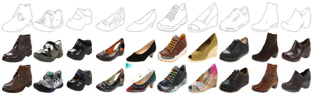
Voila! We finally have the results from the Pix2Pix model that we trained in TensorFlow. The final row represents images produced by the generator. They all look so unique and realistic. Note, how on a global level, both the generated and ground truth-images look so similar. But on a finer level, differences are evident, especially in color. This means that our generator has not learned to produce images exactly similar to the ground truth (target images). The generated images do have some randomness factor like color, while preserving the overall global structure of the object.

Here’s a fun activity for you:  Draw boundaries of a shoe you would like to generate in paint and save it as an image. Then feed it to the model, and see how well it generates a shoe for you.

Conclusion

This was an important and detailed topic and you have learned a lot, so let’s quickly summarize:

1. We introduced you to the problem of Paired Image-to-Image Translation (Pix2Pix) and discussed its various applications.
2. You learned how Paired Image-to-Image Translation works in GAN.
3. We discussed what makes Pix2Pix GAN different from the traditional GAN, and why it generates more realistic-looking images.
4. You then learned about the UNET Generator and PatchGAN Discriminator employed in Pix2Pix GAN.
5. We even discussed the Pix2Pix loss function in detail.
6. Then we implemented Pix2Pix in PyTorch, with Edges->Shoes Dataset.
7. Finally, we also implemented Pix2Pix in TensorFlow, with Multi-GPU support, on the Edges->Shoes Dataset, and achieved even better results than the PyTorch Implementation.

With Pix2Pix, you have struck a major goal. Let’s now see you race towards even bigger goals.

References

1. https://www.tensorflow.org/tutorials/generative/pix2pix
2. https://github.com/junyanz/pytorch-CycleGAN-and-pix2pix