RAFT: Optical Flow estimation using Deep Learning

In this post, we will discuss about two Deep Learning based approaches for motion estimation using Optical Flow. FlowNet is the first CNN approach for calculating Optical Flow and RAFT which is the current state-of-the-art method for estimating Optical Flow. We will also see how to use the trained model provided by the authors to perform inference on new data using PyTorch.

We cover the following topics in this article:

1. The Optical Flow Task
2. FlowNet
   1. FlowNet Architecture
   2. FlowNet Loss Function
3. RAFT
   1. RAFT Architecture
   2. Upsampling Module
   3. RAFT Loss Function
   4. RAFT and RAFTS comparison
4. RAFT inference in PyTorch
5. Model Evaluation

The Optical Flow task

In the previous post, we discussed basic components and some algorithmic approaches to estimate the Optical Flow. Let us remind you that the Optical Flow task consists of estimating per-pixel motion between two consecutive frames. Our goal is to find the displacement of a sparse feature set or all image pixels to calculate their motion vectors. An underlining theory and practical solution with OpenCV were reviewed in the previous post, and now we will continue this topic with Deep Learning approaches to the Optical Flow estimation.

FlowNet

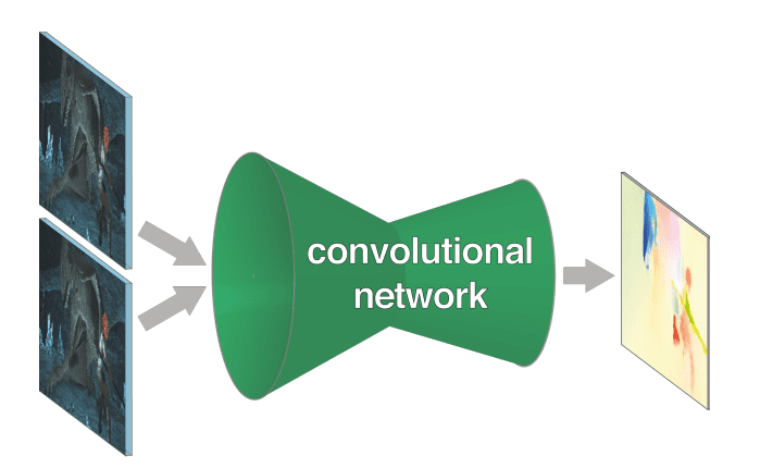
FlowNet architecture was introduced in 2015 as the first CNN approach to predict Optical Flow. Authors were inspired by the successful results of CNN architectures in classification, depth estimation, and semantic segmentation tasks. As Deep Learning approaches and CNNs have become a profitable strategy to solve many Computer Vision tasks, authors, in turn, introduced two neural networks for the Optical Flow estimation.

Architecture

FlowNetS and FlowNetCorr architectures both contain encoder and decoder parts similar to the U-Net architecture. Encoder extracts features from two consecutive images, while the decoder upscales the encoder feature maps and gets the final Optical Flow prediction. Let’s take a deeper look at both FlowNetS and FlowNetCorr networks.

FlowNetS encoder

Input data in FlowNetS (also known as FlowNetSimple) is a concatenation of two consecutive frames. These two images are places into 6-channel tensor, where the first three channels belong to the first image, the three remaining channels belong to the second image. The encoder part consists of several convolution layers followed by activation functions. This architecture allows the network to decide itself how to process two stacked images and give the feature map for the following result refinement.

FlowNetCorr encoder

The FlowNetCorr architecture takes only one frame at a time as an input, so the images are not stacked here. In this network, the authors use the first stages of CNN with shared weights to extract features from two consecutive images separately. The next step is to combine two calculated feature maps from the first and second frames respectively. To provide this, the authors introduce a new technique called Correlation layer, which is the main difference between FlowNetS and FlowNetCorr. The computation of correlation is equal to convolution operation, but there are no trainable kernels here – one feature map convolve with another. As a result, this layer performs multiplicative patch comparisons between two feature maps and has no trainable weights.

The correlation formula for two square-shaped patches centered at for the first and second feature maps respectively defined as:

The square patch size is defined as . It is important to mention that authors don’t do the full correlation between two feature maps, instead they do it patch-wise.

After the matching process of two feature maps done, the correlation result makes a forward-pass to the rest of the convolution layers to extract high-level features. The image below represents the architecture of FlowNetCorr:

FlowNetS and FlowNetCorr decoder

The output feature maps from the encoder are 64 times smaller than the input image resolution, so we need to upscale the result. The strategy here is equal for both architectures. The trainable upconvolution layers are used in the decoder stage to upscale the encoder Optical Flow output. Each decoder stage concatenates upscaled results from the previous stage and the feature map from the corresponding layer of the encoder. Using data from encoder helps with predicting the fine details like it is done in U-Net. The authors use only four stages of upscaling because using more of them provides a marginal improvement in quality. To upscale the output to the initial image resolution, it is better to use the computationally less expensive bilinear upsampling.

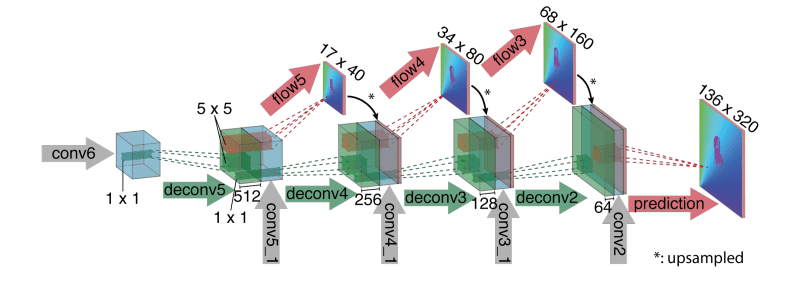
The network output is a tensor with two channels, the first one consists of motion displacement for each pixel for the x-axis, the second one – for the y-axis. As a result, we have a motion vector for every pixel in the image.

Loss function

A good penalty strategy for FlowNet is a Multi-scale training loss. The final prediction is the upscaled small-sized Optical Flow, so the small predictions have a great impact on the next large-sized ones. The loss is calculated for every decoder stage with the impact-decreasing parameter to get the fine prediction on every decoder stage. As a result, the calculated loss for a small-sized prediction has more contribution to the total loss rather than the larger one.

The loss formula for every decoder stage is based on the endpoint error between prediction and ground truth data :

RAFT

The state-of-the-art approach, according to the SINTEL benchmark, is a
composition of CNN and RNN architectures introduced in 2020. The new approach is called RAFT – Recurrent All-Pairs Field Transforms. As in the previous architecture, it also has two different types – RAFT and RAFT-S. These two architectures have a common ground, but RAFT-S is a lightweight version of the RAFT. Here we will take a look at the basic components and ideas of RAFT architecture and then compare it with the RAFT-S.

Architecture

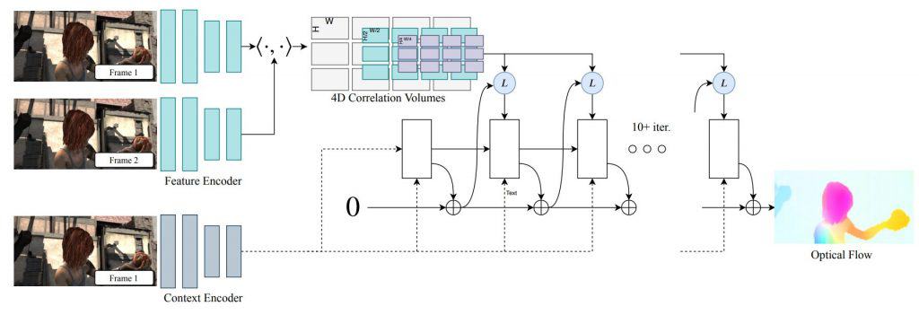
According to the paper, RAFT can be divided into three stages:

1. Feature extractors. The network input consists of two consecutive frames. To extract features from these two images, the authors use two CNNs with shared weights. This approach is similar to FlowNetCorr architecture, where we extract features from two images separately. CNN’s architecture consists of 6 residual layers, like ResNet’s layers, with the resolution reduced by half on every second layer along with an increasing number of channels. Here we can see the RAFT encoder structure:
   
   Also, the same CNN architecture is used for the Context network, which produces features only from the first image. There is only one difference in the normalization method – the feature extractor uses instance normalization while context network uses batch normalization. The Context network’s feature map will be used later in the recursive blocks.
   
   
2. Visual Similarity. Visual similarity is calculated as the inner product of all pairs of feature maps. As a result, we will have a 4D tensor called Correlation volumes that gives crucial information about small and large pixel displacements. This approach shouldn’t be confused with Correlation layer in FlowNetCorr. In FlowNetCorr we use a patch-wise correlation, while in RAFT we calculate the all-pairs correlation of two feature maps without any fixed-sized window. To be clear, the correlation is calculated between two feature maps as:
   
   
   After that, the 4-layer correlation pyramid is constructed by pooling the last two dimensions of this 4D tensor with the kernels of sizes 1, 2, 4, 8. The 2-D slices of the first three layers you can see in the picture below:
   
   
   
   The Correlation Pyramid is used to create a multi-scale image similarity features to make the abrupt movements more noticeable. Hence, the Pyramid gives information about both small and large displacements.
   
   
3. Iterative update. An iterative update is a sequence of Gated Recurrent Unit (GRU) cells that combine all data we have calculated before. GRU cells mimic an iterative optimization algorithm with the one improvement – there are trainable convolution layers with the shared weights there. One update iteration produces a new Optical Flow update to make the prediction more accurate on each new step: . The classical GRU cell scheme is represented below:
   
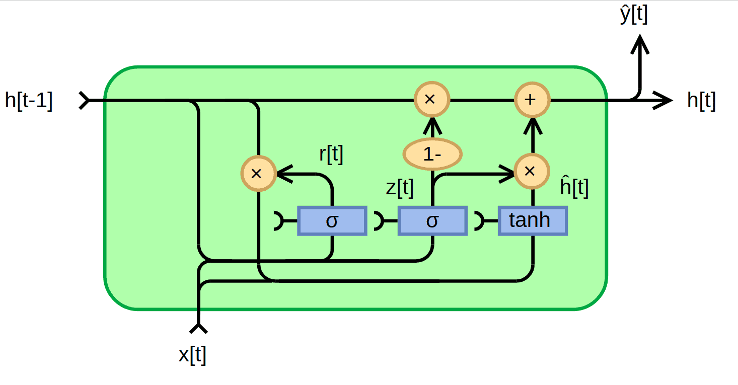   Image credits: Wikipedia
   
   These GRU cell inputs are the previous hidden state and the as the concatenation of flow, correlation, and context features. The GRU cell with convolution layers instead of fully connected layers is defined as:
   
   
   
   The authors also used only convolution layers instead of GRU block, but the results were worse in comparison with GRU. This can be explained by the fact that the convergence of the flow prediction sequence is better with the usage of gated activation. GRU cells are ideologically close with LSTM cells in recurrent networks, and you can read more about them using this link.

Upsampling module

The GRU cell outputs the Optical Flow at the 1/8 of the resolution of the initial image, so the authors propose two different ways of upsampling it to match the ground truth resolution. The first one is the bilinear interpolation of the Optical Flow. It is simple and fast approach, but the quality of this method is not as good as a learned upsample module called Convex Upsampling:

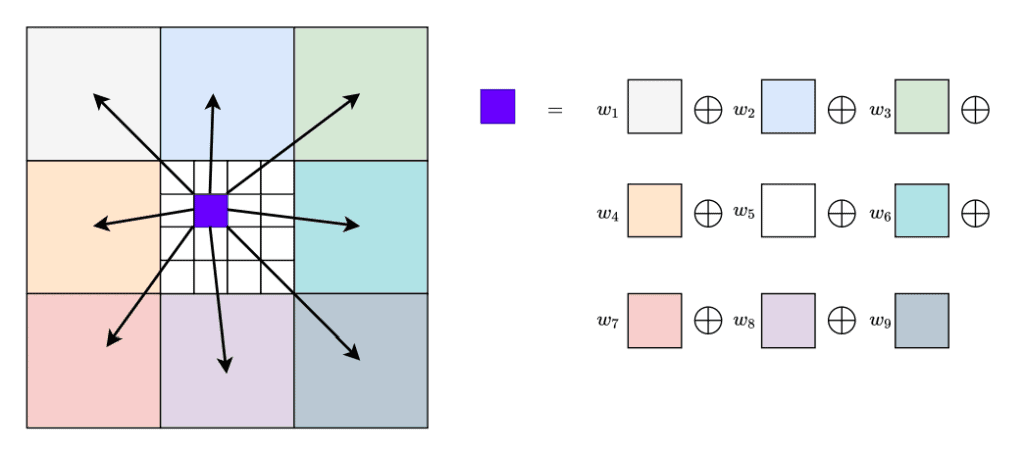
Convex Upsampling method states that the full-resolution Optical Flow is a convex combination of the weighted grid that GRU cell predicts. The 8 times image upsampling means that the one pixel must be expanded into 64 () pixels. Convex Upsampling module consists of two convolution layers and the softmax activation at the end to predict the mask for each new pixel in the upsampled Optical Flow prediction. Now, each pixel on the upsampled image is a convex combination of previous coarse resolution pixels weighted by the predicted mask with coefficients:

According to the authors, this method predicts more accurate Optical flow output, particularly near motion boundaries.

Loss function

The loss function is defined as the L1 distance between ground truth and prediction, equal to the loss in FlowNet. All upsampled recurrent cell outputs create a sequence of the Optical Flow predictions .

The total loss is the sum of losses on each recurrent block output between the ground truth and the upsampled prediction:

RAFT & RAFT-S comparison

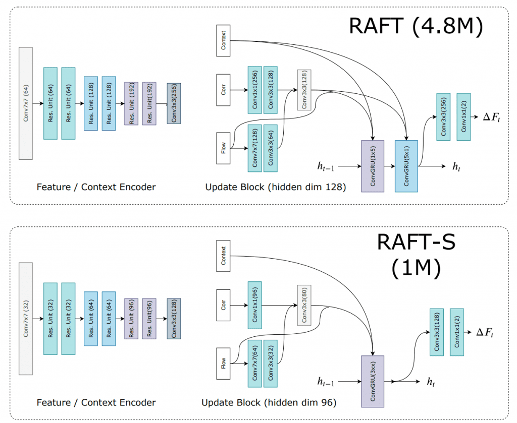
As we mentioned before, the two types of network architecture were introduced in the original paper – RAFT and RAFT-S. Let’s take a look at the graphical comparison of them:

Firstly, the Feature and Context Extractor has a different number of channels, and in RAFT-S the residual units are replaced with bottleneck residual units. Secondly, the RAFT architecture has two convolution GRU cells in one block with and kernel sizes, while RAFT-S has only one convolution GRU cell. As a result, RAFT-S, the lightweight version of the RAFT, has less number of parameters while being a bit less accurate in terms of quality.

You can find the README.md file related to this post in Optical-flow-as-a-deep-learning task folder.

RAFT with PyTorch

The authors also attach the open-source implementation of the RAFT architecture with pretrained weights. This is great, so we can check this architecture and create our inference script using the author’s developments. To start the demo, you need to download our code and install the required libraries. All the info about installation you can find in README.md file.

Now, let’s take a look at the code part of the inference script. At first, we need to define the model and load pretrained weights:

def inference(args):
    # get the RAFT model
    model = RAFT(args)
    # load pretrained weights
    pretrained_weights = torch.load(args.model)

Click here to download the source code to this post

To run inference for both CPU and GPU devices, we need to check the GPU availability. By default, the script uses your CPU device:

if torch.cuda.is_available():
    device = "cuda"
    # parallel between available GPUs
    model = torch.nn.DataParallel(model)
    # load the pretrained weights into model
    model.load_state_dict(pretrained_weights)
    model.to(device)
else:
    device = "cpu"
    # change key names for CPU runtime
    pretrained_weights = get_cpu_model(pretrained_weights)
    # load the pretrained weights into model
    model.load_state_dict(pretrained_weights)

The pretrained model was trained on two GPUs with torch.nn.DataParallel, so the dictionary keys in the pretrained model have additional prefix name module. To run inference on CPU, we need to remove this prefix and get the new CPU-suitable model:

def get_cpu_model(model):
    new_model = OrderedDict()
    # get all layer's names from model
    for name in model:
        # create new name and update new model
        new_name = name[7:]
        new_model[new_name] = model[name]
    return new_model

Now, we can go forward with our demo task. This part of the code reads two consecutive frames and then outputs the Optical Flow prediction. After that, we encode flow prediction and convert it into a BGR image.

with torch.no_grad():
    while True:
        # read the next frame
        ret, frame_2 = cap.read()
        if not ret:
            break

        # preprocessing
        frame_2 = frame_preprocess(frame_2, device)

        # predict the flow
        flow_low, flow_up = model(frame_1, frame_2, iters=20, test_mode=True)

        # vusialize the results
        ret = vizualize_flow(frame_1, flow_up, save, counter)
        if not ret:
            break
        frame_1 = frame_2
        counter += 1

To visualize the flow, we use the standard RAFT’s encoder. The visualization strategy is almost similar to the HSV we used in the previous post. After we get Optical Flow result in BGR format, we concatenate the image and Optical Flow for visualization:

def vizualize_flow(img, flo, save, counter):
    # convert CWH to WHC format and change device if necessary  
    img = img[0].permute(1, 2, 0).cpu().numpy()
    flo = flo[0].permute(1, 2, 0).cpu().numpy()

    # map flow to rgb image
    flo = flow_viz.flow_to_image(flo)
    flo = cv2.cvtColor(flo, cv2.COLOR_RGB2BGR)

    # concatenate, save and show images
    img_flo = np.concatenate([img, flo], axis=0)
    if save:
        cv2.imwrite(f"demo_frames/frame_{str(counter)}.jpg", img_flo)
    cv2.imshow("Optical Flow", img_flo / 255.0)

    k = cv2.waitKey(25) & 0xFF
    if k == 27:
        return False
    return True

To run the demo you can use this command:

python3 inference.py --model=./models/raft-sintel.pth --video ./videos/crowd.mp4

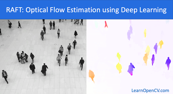
The code runtime will give you the inference window with video and flow prediction:

Models evaluation

Metric: End-point error

The standard error measure for the Optical Flow task is called End-point error and defined as the Euclidean distance between ground-truth and calculated Optical Flow values for each pixel in the image (for the case of the dense Optical Flow estimation). As you may see, the metric and the loss function for FlowNet and RAFT are equal:

Benchmarks

There are some open-source Optical Flow datasets and benchmarks that depict the predominance of Deep Learning solutions over the classical ones in terms of quality and inference time. One of the most famous datasets is the SINTEL dataset, which has its own benchmark. The FlowNet architecture has quite good results, but it still worse than some algorithmic approaches like DeepFlow and EpicFlow. Regarding the RAFT architecture, it takes the first place in SINTEL benchmark. You can compare the visualization of results by RLOF method, which we reviewed in the previous post, and the state-of-the-art RAFT architecture.

Also, there is a KITTY benchmark, where RAFT takes the third place, still being better than any other algorithmic approach.

Conclusion

Optical Flow finds it’s application in many tasks of video editing like stabilization, compression, slow-motion, and so on. Moreover, some tracking and action-recognition systems also use Optical Flow data. In this post, we reviewed some Deep Learning approaches that gave a quality boost on the example of FlowNet and RAFT architectures. Nowadays, RAFT architecture shows the best result on the SINTEL dataset and top-3 on the KITTY dataset.