
In the constantly evolving field of computer vision, understanding the precise structure and pose of objects is essential. Whether it’s detecting a specific object in a cluttered scene or analyzing human postures in real time, keypoints play a crucial role. These distinctive points on an object, often corresponding to the corners, edges, or other recognizable parts, serve as anchors to identify and track the object. But how can we measure the similarity and precision of these detected keypoints? Enter the concept of Object Keypoint Similarity (OKS), a specific metric used to gauge the accuracy of keypoint detection. OKS provides a standardized way to compare the predicted keypoints with the ground truth, considering factors such as scale, unlabelled keypoints and ambiguity in annotations.
This post will address some of the most frequently asked questions: What is Object Keypoint Similarity (OKS)? How is OKS calculated? How does OKS handle different scales and object sizes?
- Intersection over Union in Object Detection
- Object Keypoint Similarity (OKS) in Keypoint Detection
- Pitfalls of using only Euclidean distances as a Similarity Measure
- Significance of Per-keypoint Standard Deviation (Sigmas) during OKS Computation
- Implementation of Object Keypoint Similarity
- Conclusion
- References
Intersection over Union in Object Detection
Before we dive deeper into Object Keypoint Similarity, it is imperative to have a basic understanding of Intersection Over Union (IoU) in object detection. Broadly speaking, IoU helps estimate the similarity measure between 2 bounding boxes. Mathematically, it is defined as the ratio between the intersection area to the union area of two bounding box instances.
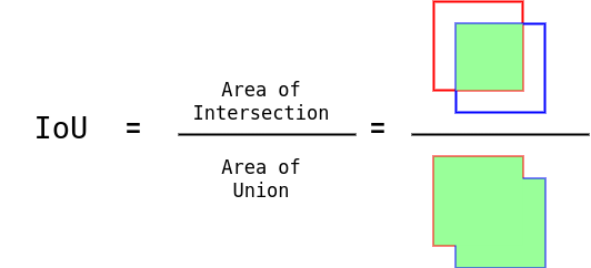
IoU lies in the range [0, 1]. An IoU score of 1 indicates a perfect overlap, while an IoU score of 0 indicates no overlap. A high IoU score establishes a strong similarity across the corresponding bounding boxes.
IoU becomes the essence for the evaluation metrics in object detection, such as mean Average Precision(mAP) and Average Recall (AR), since it provides the estimate of the similarity measure between ground truth and predicted object instances.
We have an in-depth post on Intersection over Union that will help you gain a deeper understanding of the subject.
Object Keypoint Similarity (OKS) in Keypoint Detection
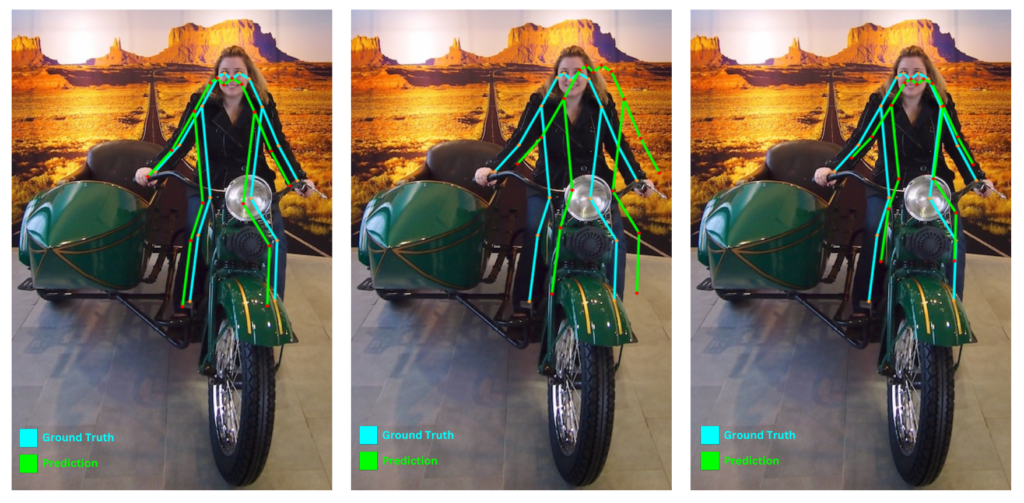
Consider the image shown below depicting the ground truth keypoints (cyan) and predicted keypoints (green) from 3 models on human pose.
Similar to IoU, we can also establish a similarity measure between the ground truth and predicted keypoint sets.
We can observe the following:
- The predicted set of keypoints from the first model (left) is very close to that of the ground truth counterparts.
- The predicted set of keypoints from the second model (middle) is distant from the ground truth.
- The predicted set of keypoints from the third model (right) is close to the ground truth but somewhat scaled.
Intuitively, we can guess that the predicted keypoint from the first model should have the highest similarity score, followed by that of the third model, and lastly, the second model.
Unlike IoU, which is an area-based computation, for keypoints, a distance-based approach needs to be established. Hence, MS-COCO proposed object keypoint similarity (OKS) as a means to establish a similarity measure between two sets of keypoints.
Keypoint similarity (KS) is calculated in a per-keypoint fashion. It is computed by passing the Euclidean distance between the ground truth and predicted keypoint over an un-normalized Gaussian distribution with standard deviation ski, where s is the scale, which is basically the square root of the object’s segmented area, and k is the per-keypoint constant.
Mathematically, the keypoint similarity for keypoint type i is given as:

where,
- di is the Euclidean distance between the ground truth and predicted keypoint i
- k is the constant for keypoint i
- s is the scale of the ground truth object; s2 hence becomes the object’s segmented area.
For each keypoint, the KS lies between 0 and 1.
COCO specifies that each ground truth annotated keypoint should have a visibility flag. The visibility flag can assume either of the three values:
0: indicates an unlabeled keypoint1: indicates that the keypoint is labeled but not visible2: indicates that the keypoint is labeled and visible
Object keypoint similarity (OKS) is finally computed as the arithmetic average across all labeled keypoints in an instance.
The mathematical notation for OKS is given by:

where:
- KSi is the keypoint similarity for keypoint type
i - vi is the ground truth visibility flag for keypoint
i - δ(vi > 0) is the Dirac-delta function which computes as
1if the keypointiis labeled, otherwise0
ki was tuned by measuring the per-keypoint standard deviation ![]() with respect to the object scale using the 5000 redundantly annotated images in the validation data.
with respect to the object scale using the 5000 redundantly annotated images in the validation data.
Finally, the setting: ki = 2 σi was used as the per-keypoint constant in COCO.
The per-keypoint standard deviation (![]() ) across all 17-COCO pose landmarks is provided in the table below.
) across all 17-COCO pose landmarks is provided in the table below.
| Keypoints | δi |
| Nose | 0.026 |
| Eyes | 0.025 |
| Ears | 0.035 |
| Shoulders | 0.079 |
| Elbows | 0.072 |
| Wrists | 0.062 |
| Hips | 0.107 |
| Knees | 0.087 |
| Ankles | 0.089 |
In the image above, the OKS scores for each of the 3 models were 0.78, 0.38, and 0.59 (left to right), respectively, which was on expected lines.
The determination of True Positives, False Positives, and False Negatives is decided on the basis of the OKS threshold, similar to the one with IoU.
- If the OKS score between the ground truth and the prediction lies above the OKS threshold, then the detection is counted as a True Positive, while the ground truth is considered a match.
- Otherwise, the detection is counted as a False Positive.
- All unmatched ground truths are taken as False Negatives.
Similar precision and recall values are computed, followed by the final mean Average Precision (mAP) metric computation as in object detection.
Pitfalls of using only Euclidean Distances as a Similarity Measure
Using naive Euclidean distance as a similarity measure has the following downsides:
- Scale Invariance: Euclidean distance does not account for scale differences between objects. As a result, equal-sized errors for small and large objects would be misappropriately weighted.
- Robustness of keypoints not labeled in image: In practical applications, the label of a keypoints may be absent from an image, influenced by factors such as occlusion, distinct poses, or inherent characteristics of the image acquisition process. For pose estimation models, it is imperative to ensure that the evaluation metrics neither unfairly reward nor penalize the model’s ability or inability to identify these unlabeled keypoints.
- Ambiguity in Annotation: In instances where annotations for identical keypoints vary across different images, the model may face unwarranted penalties. This inconsistency poses a heightened challenge for smaller objects, as they are inherently more difficult to annotate uniformly.
Significance of Per-keypoint Standard Deviation (Sigmas) during Object Keypoint Similarity (OKS) Computation
In the previous section, we mentioned that per-keypoint constant ki was tuned by measuring the per-keypoint standard deviation σi with respect to the object scale.
The standard deviation (σi) varies substantially for different keypoints. For instance, keypoints on a person’s body (shoulders, knees, hips, etc.) tend to have a σ much larger than on a person’s head (eyes, nose, ears).
The image below depicts the keypoint similarity distribution and its representation (using concentric circles) on the image plane between the detected keypoints of the eye (red) and wrist (green) with their corresponding ground truth annotation (blue).
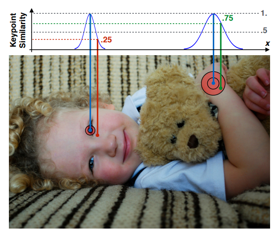
Since the σ for the keypoint of the eye is less compared to that of the wrist, the area of the circle for ks score of 0.5 for the eye is less than that of the wrist (the outer circle). The inner concentric circle for the keypoint of the wrist signifies a keypoint-similarity score of 0.85. The image also highlights that even though the distances between the ground truth and detected keypoints for both the eye and the wrist are identical, the keypoint similarity scores turn out to be 0.25 and 0.75, respectively. This is because the sigma for the wrist is comparatively large than that of the eye.
One might also be intrigued why not assign the keypoint score across all keypoints equally, more specifically, by assigning each of them with probability scores sampled from a uniform distribution (determined by the total number of keypoints) equally.
It turns out that this may work well if the number of keypoints is significantly large, but it might not be a good idea if we are provided with a fewer number of keypoints.
In the next section, we will discuss more the effect of the choice of sigmas on the OKS scores.
Implementation of Object Keypoint Similarity
The function keypoint_similarity below shows the implementation of OKS.
def keypoint_similarity(gt_kpts, pred_kpts, sigmas, areas):
    """
    Params:
        gts_kpts: Ground-truth keypoints, Shape: [M, #kpts, 3],
                  where, M is the # of ground truth instances,
                         3 in the last dimension denotes coordinates: x,y, and visibility flag

        pred_kpts: Prediction keypoints, Shape: [N, #kpts, 3]
                   where  N is the # of predicted instances,

        areas: Represent ground truth areas of shape: [M,]

    Returns:
        oks: The Object Keypoint Similarity (OKS) score tensor of shape: [M, N]
    """

    # epsilon to take care of div by 0 exception.
    EPSILON = torch.finfo(torch.float32).eps

    # Eucleidian dist squared:
    # d^2 = (x1 - x2)^2 + (y1 - y2)^2
    # Shape: (M, N, #kpts) --> [M, N, 17]
    dist_sq = (gt_kpts[:,None,:,0] - pred_kpts[...,0])**2 + (gt_kpts[:,None,:,1] - pred_kpts[...,1])**2

    # Boolean ground-truth visibility mask for v_i > 0. Shape: [M, #kpts] --> [M, 17]
    vis_mask = gt_kpts[..., 2].int() > 0

    # COCO assigns k = 2σ.
    k = 2*sigmas

    # Denominator in the exponent term. Shape: [M, 1, #kpts] --> [M, 1, 17]
    denom = 2 * (k**2) * (areas[:,None, None] + EPSILON)

    # Exponent term. Shape: [M, N, #kpts] --> [M, N, 17]
    exp_term = dist_sq / denom

    # Object Keypoint Similarity. Shape: (M, N)
    oks = (torch.exp(-exp_term) * vis_mask[:, None, :]).sum(-1) / (vis_mask[:, None, :].sum(-1) + EPSILON)

    return oks
It accepts the following arguments:
gts_kpts: Ground-truth keypoints having shape:[M, #kpts, 3], where,Mis the number of ground truth instances, and3in the last dimension denotes coordinates: x,y, and visibility flag.pred_kpts: Prediction keypoints having shape:[N, #kpts, 3]where,Nis the number of predicted instances,sigmas: The per-keypoint standard deviations.areas: Represent ground truth areas of shape:[M,]
An implementation note: As mentioned earlier, area (or s2) is the object’s segmented area and not the bounding box area. In cases where only the bounding box data, such as the width and height, is available, the segmented area can be approximated by heuristically multiplying a scaling factor of 0.53 with the bounding box area.
The function draw_keypoints is for visualizing the keypoints given an image. The implementation is shown below.
def draw_keypoints(image, keypoints, lm_color=(0,255,0), edge_color=(0,255,0)):

    image = image.copy()

    radius = 2

    EDGES = [(0,1), (0,2), (1,3), (2,4), (3,5), (4,6), (5,7), (6,8),
             (7,9), (8,10), (5,11), (6,12), (11,13), (12,14), (13,15), (14,16)]

    for edge in EDGES:
        src_x, src_y   = keypoints[edge[0]].astype("int").tolist()
        dest_x, dest_y = keypoints[edge[1]].astype("int").tolist()
        cv2.line(image, (src_x, src_y), (dest_x, dest_y), color=edge_color, thickness=2, lineType=cv2.LINE_AA)

    for idx, coords in enumerate(keypoints):

        loc_x, loc_y = coords.astype("int").tolist()

        cv2.circle(image,
                   (loc_x, loc_y),
                   radius,
                   color=lm_color,
                   thickness=-1,
                   lineType=cv2.LINE_AA)


    return image
Let us take the following image with ground truth (cyan) and predicted keypoints (green).

The ground truth annotation is specified in the block below.
gt_kpts_1 = torch.tensor([[292, 93,  2],
                          [303, 84,  2],
                          [283, 84,  2],
                          [316, 92,  2],
                          [274, 90,  2],
                          [333, 129, 2],
                          [253, 128, 2],
                          [355, 181, 2],
                          [223, 180, 2],
                          [380, 227, 2],
                          [191, 215, 2],
                          [318, 251, 1],
                          [264, 250, 2],
                          [353, 307, 2],
                          [248, 300, 2],
                          [350, 387, 1],
                          [237, 388, 2]], dtype = torch.float)
The detections are generated by translating them to X, Y = [-10, 7] pixels. Hence the effective distance between them is ![]() = 12.20 pixels.
= 12.20 pixels.
det_kpts_1 = gt_kpts_1.clone()
det_kpts_1[:, :2]+= torch.tensor([-10, 7])
Since we are dealing with COCO keypoints, we set it accordingly.
NUM_KPTs = 17
We also set the area of this instance as provided in COCO’s validation data.
areas = torch.tensor([30699.56495])
Per-Keypoint Standard Deviations Initialized from COCO
Let us initialize the sigmas in accordance with COCO mentioned earlier.
KPTS_OKS_SIGMAS_COCO = torch.tensor([.26, .25, .25, .35, .35, .79, .79, .72, .72, .62,.62, 1.07, 1.07, .87, .87, .89, .89])/10.0
We compute the OKS score by passing the required arguments to the keypoint_similarity function.
oks_coco = keypoint_similarity(gt_kpts_1.unsqueeze(0),
                               det_kpts_1.unsqueeze(0),
                               sigmas=KPTS_OKS_SIGMAS_COCO,
                               areas=areas)
The OKS score turns out to be: 0.7812.
Per-Keypoint Standard Deviations Sampled from Uniform Distribution
Let us now initialize the sigmas sampled from a uniform distribution with a probability score of 1/ #kpts.
KPTS_OKS_SIGMAS_UNIF = torch.ones(NUM_KPTs)/NUM_KPTs
Let us compute the OKS score as well.
oks_unf_sigma = keypoint_similarity(gt_kpts_1.unsqueeze(0),
                                    det_kpts_1.unsqueeze(0),
                                    sigmas=KPTS_OKS_SIGMAS_UNIF,
                                    areas=areas)
The OKS score comes out to be 0.8392, which is comparatively higher than the one initialized COCO sigmas.
This would cause the evaluation metrics for keypoint detection to be higher. Therefore, one needs to be careful with the choice of sigmas while performing training in keypoint detection.
The keypoint sigmas assigned with uniform probability scores may still produce decent results when the number of keypoints is significant. However, this is also subject to experimentation.
Effect of Euclidean Distance on Object Keypoint Similarity (OKS) for Large Objects
Let us now compute the OKS score by translating the ground truth keypoints to X, Y = [12.5, 5].
det_kpts_2 = gt_kpts_1.clone()
det_kpts_2[:, :2]+= torch.tensor([12.5, 5])
The OKS between `det_kpts_2` and `gt_kpts_1` turns out to be 0.7481 (using COCO sigmas).
From the OKS values above, one can observe that the effective distance was increased from ![]() pixels to
pixels to ![]() pixels. Although the OKS score has decreased, which was expected, this distance increase did not have a significant bearing on the OKS score. This is primarily attributed to the scale factor (the object area of which was
pixels. Although the OKS score has decreased, which was expected, this distance increase did not have a significant bearing on the OKS score. This is primarily attributed to the scale factor (the object area of which was 30699.57 pixels), which is quite significant here.
Effect of Euclidean Distance on Object Keypoint Similarity (OKS) for Small Objects
Let us take a look at another sample where we have a smaller object.

The ground truth pose edges are represented with cyan, while that of the detection is represented in green.
The segmented area of the instance is 1576.46 pixels.
The detections were generated by translating the ground truth keypoints to [5, 3].
det_kpts_3 = gt_kpts_2.clone()
det_kpts_3[:, :2]+= torch.tensor([5, 3])
The OKS values with COCO and Uniform sigmas are: 0.4794 and 0.4588, respectively.
Recall that in our previous example, the object scale was relatively higher compared to the current example. Therefore, the scale has a dominating effect on large objects as well. However, with small objects, the scale shares an equal contributing factor with the sigma scores.
Finally, we shall translate the ground truth boxes to X, Y = [6, 3.77] pixels and use them as our detections such that the effective distance becomes ![]() = 7.086 pixels.
= 7.086 pixels.
det_kpts_4 = gt_kpts_2.clone()
det_kpts_4[:, :2]+= torch.tensor([6, 3.77])
The OKS scores with COCO and Uniform sigmas turn out to be 0.3872 and 0.3164, respectively.
We can see that although the effective distance changes from ![]() pixels to
pixels to ![]() pixels, the OKS score reduces significantly!
pixels, the OKS score reduces significantly!
The object’s diminutive scale is the key reason behind this.
Conclusion
So far in this article, we have tried to develop the notion of Object Keypoint Simiarity as a similarity measure between two sets of keypoints. Furthermore, the following conclusions can be drawn from the results:
- OKS varies significantly for small objects even when the relative distance between the two sets of keypoints varies slightly. This logic, however, doesn’t hold good for larger objects.
- The area of the object instance can have a dominant factor for large objects in the OKS score compared to small objects.
- The choice while determining the per-keypoint standard deviations play a crucial role while computing the OKS score.
Analogous to object detection, where the IoU between the ground truth and the detection can be used a loss function during training, a similar corollary can be drawn while using OKS as a loss function.
References
- Ultralytics Repository
- Extended COCO API (xtcocotools)
- Benchmarking and Error Diagnosis in Multi-Instance Pose Estimation
- ICCV17 – Keypoints Overview




100K+ Learners
Join Free OpenCV Bootcamp3 Hours of Learning