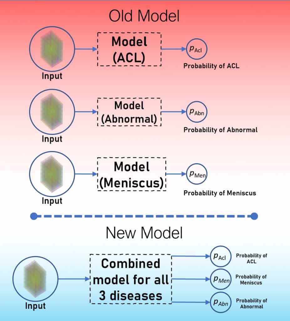
Our last post on the MRNet challenge presented a simple way to approach it. There you learned to make a separate model for each disease. And ended up with three models.
Time to up your game! Now combine all the three models into one and train it.
- The Combined Model Approach
- Intro to some changes in the model
- Advantages
- Results
- Further improvements
- Conclusion
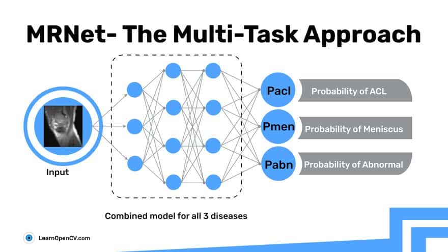
The Combined Model Approach – Multitask
But why multitask? That’s a valid question.
Multitask learning is actually inspired by human learning. When learning new tasks, don’t you tend to apply the knowledge gained when learning related tasks. For instance, a baby first learns to recognize faces, then applies the same technique perhaps to recognize other objects.
Babies have a mind of their own, you might say. Okay, so let’s take the example of a superhero. Just imagine your favorite superhero character training to become stronger. No, he’s not lifting weights or directly practicing to fight. May be he performs some other auxiliary tasks, unrelated to fighting. But in hindsight, these go on to equip him with skills and muscle to get stronger. (For the anime fans out there, think of Naruto while training to master Rasengan)
Am sure you also learnt to do simple stuff first, then applied the learning from it to graduate to more complex techniques.
The same logic shall drive you to adopt a multitask approach in this challenge. Let’s start with the assumption that a model will be able to predict Disease A better, if it is already experienced in recognizing Disease B. Perhaps it can trace similar patterns. Or maybe, there was a part of the knee that the model overlooked while looking for Disease A, but does not miss in Disease B. And that helps in detection of Disease A.
Also, as the losses of all three diseases propagate throughout the model, they start supporting each other in detection, due to the similarity of their tasks.
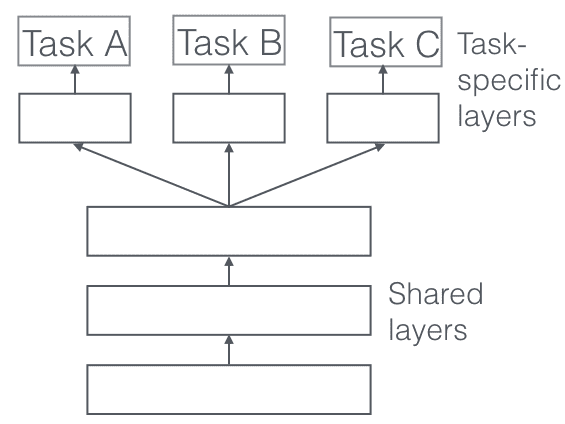
The following multi-task approach is called Hard Parameter Sharing. In this, you share the hidden layers between all tasks, while keeping several task-specific output layers.
Keen to dig deeper in Multitask learning? Check out this paper by Sebastian Ruder. Quoting a line from this paper to sum up this section:
Hard Parameter Sharing greatly reduces the risk of overfitting. In fact, it was shown that the risk of overfitting the shared parameters is an order N — where N is the number of tasks — smaller than overfitting the task-specific parameters, i.e. the output layers. This makes sense intuitively: The more tasks we are learning simultaneously, the more our model has to find a representation that captures all of the tasks, and the less is our chance of overfitting on our original task.
Changes Introduced
Going from a single-disease model to a multi-disease model required not much change. Here are the main changes we made to get to it:
Dataloader
Just one small change in the data loader. Instead of providing a single label for that one disease, you now provide a tensor of size 3 that contains labels for all three diseases. The image provided across all 3 planes remains the same as the one in the single-disease models.
class MRData():
    """This class used to load MRnet dataset from `./images` dir
    """

    def __init__(self,task = 'acl', train = True, transform = None, weights = None):
        """Initialize the dataset
        Args:
            plane : along which plane to load the data
            task : for which task to load the labels
            train : whether to load the train or val data
            transform : which transforms to apply
            weights (Tensor) : Give wieghted loss to postive class eg. `weights=torch.tensor([2.223])`
        """
        self.planes=['axial', 'coronal', 'sagittal']
        self.records = None
        # an empty dictionary
        self.image_path={}

        if train:
            self.records = pd.read_csv('./images/train-{}.csv'.format(task),header=None, names=['id', 'label'])

            '''
            self.image_path[<plane>]= dictionary {<plane>: path to folder containing
                                                                image for that plane}
            '''
            for plane in self.planes:
                self.image_path[plane] = './images/train/{}/'.format(plane)
        else:
            transform = None
            self.records = pd.read_csv('./images/valid-{}.csv'.format(task),header=None, names=['id', 'label'])
            '''
            self.image_path[<plane>]= dictionary {<plane>: path to folder containing
                                                                image for that plane}
            '''
            for plane in self.planes:
                self.image_path[plane] = './images/valid/{}/'.format(plane)


        self.transform = transform

        self.records['id'] = self.records['id'].map(
            lambda i: '0' * (4 - len(str(i))) + str(i))
        # empty dictionary
        self.paths={}
        for plane in self.planes:
            self.paths[plane] = [self.image_path[plane] + filename +
                          '.npy' for filename in self.records['id'].tolist()]

        self.labels = self.records['label'].tolist()

        pos = sum(self.labels)
        neg = len(self.labels) - pos

        # Find the wieghts of pos and neg classes
        if weights:
            self.weights = torch.FloatTensor(weights)
        else:
            self.weights = torch.FloatTensor([neg / pos])

        print('Number of -ve samples : ', neg)
        print('Number of +ve samples : ', pos)
        print('Weights for loss is : ', self.weights)

    def __len__(self):
        """Return the total number of images in the dataset."""
        return len(self.records)

    def __getitem__(self, index):
        """
        Returns `(images,labels)` pair
        where image is a list [imgsPlane1,imgsPlane2,imgsPlane3]
        and labels is a list [gt,gt,gt]
        """
        img_raw = {}

        for plane in self.planes:
            img_raw[plane] = np.load(self.paths[plane][index])
            img_raw[plane] = self._resize_image(img_raw[plane])

        label = self.labels[index]
        if label == 1:
            label = torch.FloatTensor([1])
        elif label == 0:
            label = torch.FloatTensor([0])

        return [img_raw[plane] for plane in self.planes], label
Change in Model and Forward Pass
Your next target is to predict labels for all three diseases. So, it makes sense to have 3 output neurons instead of one. Make this one change, and end up with a fully-connected layer of 3 neurons.
Forward functions remain intact.
class MRnet(nn.Module):
    """MRnet uses pretrained resnet50 as a backbone to extract features"""

    def __init__(self): # add conf file

        super(MRnet,self).__init__()

        # init three backbones for three axis
        self.axial = models.alexnet(pretrained=True).features
        self.coronal = models.alexnet(pretrained=True).features
        self.saggital = models.alexnet(pretrained=True).features

        self.pool_axial = nn.AdaptiveAvgPool2d(1)
        self.pool_coronal = nn.AdaptiveAvgPool2d(1)
        self.pool_saggital = nn.AdaptiveAvgPool2d(1)

        self.fc = nn.Sequential(
            nn.Linear(in_features=3*256,out_features=1)
        )

    def forward(self,x):
        """ Input is given in the form of `[image1, image2, image3]` where
        `image1 = [1, slices, 3, 224, 224]`. Note that `1` is due to the
        dataloader assigning it a single batch.
        """

        # squeeze the first dimension as there
        # is only one patient in each batch
        images = [torch.squeeze(img, dim=0) for img in x]

        image1 = self.axial(images[0])
        image2 = self.coronal(images[1])
        image3 = self.saggital(images[2])

        image1 = self.pool_axial(image1).view(image1.size(0), -1)
        image2 = self.pool_coronal(image2).view(image2.size(0), -1)
        image3 = self.pool_saggital(image3).view(image3.size(0), -1)

        image1 = torch.max(image1,dim=0,keepdim=True)[0]
        image2 = torch.max(image2,dim=0,keepdim=True)[0]
        image3 = torch.max(image3,dim=0,keepdim=True)[0]

        output = torch.cat([image1,image2,image3], dim=1)

        output = self.fc(output)
        return output
Change in Loss Function and Weights
Even the loss function does not change much. You now have an output vector of size 3. Compare it with a ground-truth vector of size 3 to calculate the loss. Here again you can use Binary Cross Entropy Loss. But now that you have 3 independent classes, pass 3 +ve weights to the loss function in order to handle data imbalance across 3 diseases.
# Here train_wts are actually train_data.weights defined in the MRData class above, which is a size 3 tensor
criterion = torch.nn.BCEWithLogitsLoss(pos_weight=train_wts)
Train loop and Eval loop
Train and validation loops are the same, except you now collect AUC scores for all three diseases instead of just one.
def _train_model(model, train_loader, epoch, num_epochs, optimizer, criterion, writer, current_lr, log_every=100):

    # Set to train mode
    model.train()

    y_probs = []
    y_gt = []
    losses = []

    for i, (images, label) in enumerate(train_loader):
        optimizer.zero_grad()

        if torch.cuda.is_available():
            images = [image.cuda() for image in images]
            label = label.cuda()

        output = model(images)

        loss = criterion(output, label)
        loss.backward()
        optimizer.step()

        loss_value = loss.item()
        losses.append(loss_value)

        probas = torch.sigmoid(output)

        y_gt.append(int(label.item()))
        y_probs.append(probas.item())

        try:
            auc = metrics.roc_auc_score(y_gt, y_probs)
        except:
            auc = 0.5

        writer.add_scalar('Train/Loss', loss_value,
                          epoch * len(train_loader) + i)
        writer.add_scalar('Train/AUC', auc, epoch * len(train_loader) + i)

        if (i % log_every == 0) & (i > 0):
            print('''[Epoch: {0} / {1} | Batch : {2} / {3} ]| Avg Train Loss {4} | Train AUC : {5} | lr : {6}'''.
                  format(
                      epoch + 1,
                      num_epochs,
                      i,
                      len(train_loader),
                      np.round(np.mean(losses), 4),
                      np.round(auc, 4),
                      current_lr
                  )
                  )

    writer.add_scalar('Train/AUC_epoch', auc, epoch + i)

    train_loss_epoch = np.round(np.mean(losses), 4)
    train_auc_epoch = np.round(auc, 4)

    return train_loss_epoch, train_auc_epoch
Above is the train loop. Validation loop is similar.
Advantages
- Lessens the training time. As you’re training a single model for all three diseases, the training time reduces to one-third.
- Faster saturation is seen in the AUC score of some diseases, when trained this way.
- Less space taken, you need to store just one model instead of three. It gets easy to port the model for inferencing and allows faster inference time.
Our Results
This approach fetched decent results, achieving an average AUC of 89.43. Find below our best AUC (on validation set) scores for all the three diseases
- ACL = 0.9599
- Abnormal = 0.939
- Meniscus = 0.783
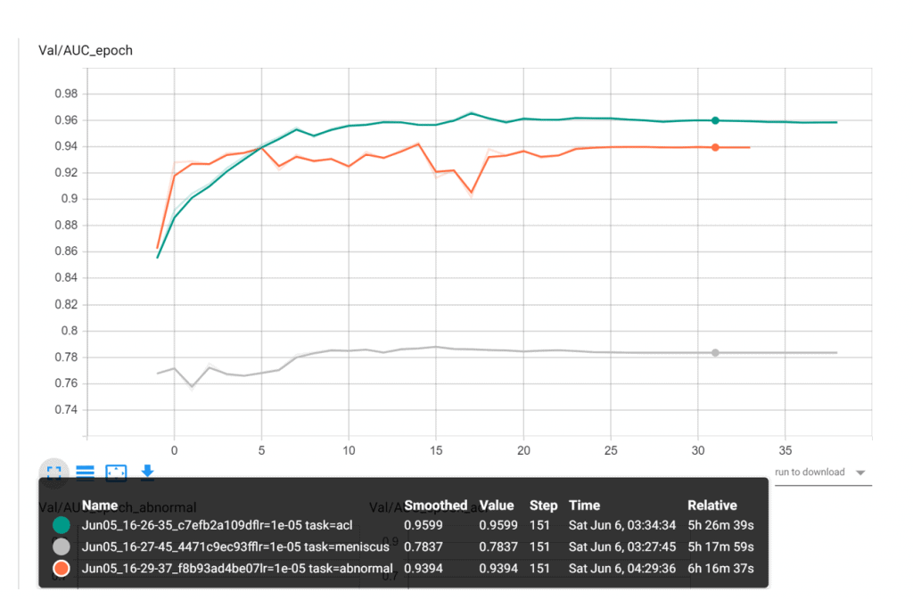
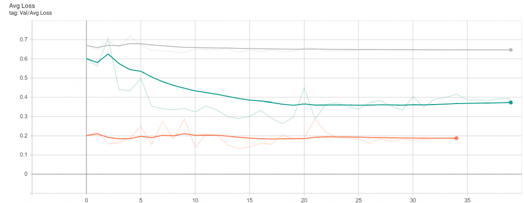
The decent increase in the AUC is followed by a steady decrease in the validation loss.
How to improve this?
Some paths still lie unexplored. They are similar to what you did in the previous blog. Want to give it a shot? Here they are:
- Use a different backbone, maybe Resnet-50 or VGG-16
- Try different/more augmentations of the MRI scans
- Train with an SGD optimizer instead of Adam
- Train for more epochs
Happy exploring! Do keep us updated on your wins.
Conclusion
- You got familiar with the MRNet Challenge Dataset and its tasks.
- Discussed what makes this dataset different from other image-classification datasets.
- You then trained 3 different models to classify MRI scans for each disease.
- Even discussed alternate approaches.
We hope you downloaded the code, so you have a hands-on experience along with following the content. We have provided detailed instructions there, so you can start training your models in no time.
Until next time ? next dataset…next challenge!
References
[ 1 ] https://stanfordmlgroup.github.io/competitions/mrnet/





100K+ Learners
Join Free OpenCV Bootcamp3 Hours of Learning