Introduction to Monocular SLAM: Have you ever wondered how Tesla’s Autonomous Vehicle views its surroundings and understands its position, and makes smart decisions to reach its target location?
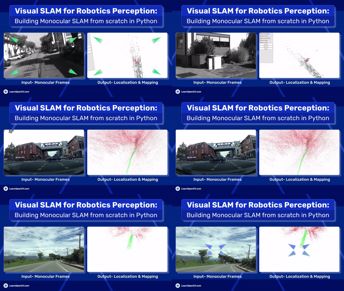
Well, the method it uses is called SLAM. Hold your horses! Before you get excited, it’s not about robots getting into wrestling matches or slamming someone to the ground.
Simultaneous Localization and Mapping, or SLAM is a well-known term in Robotics and 3D Computer Vision. It is an integral part of robotics perception, responsible for enabling robots to navigate unknown terrains. Simultaneous Localization and Mapping or SLAM in short, is a method of localizing a robot within an unknown environment.
This is part 2 of our robotics article series. In the previous blog post, we gave an in-depth overview of the Four Components of an Autonomous Robot. In this article, we’ll only focus on the perception module, specifically localization. We’ll go through Monocular Visual SLAM step by step and implement a simple version in Python OpenCV. We’ll break down all the mathematical parts to make it easier to understand. Later, we’ll briefly discuss ORB-SLAM and how to run it. For a complete overview, check out the TOC.
- What is SLAM?
- What is Visual SLAM?
- What is Monocular SLAM?
- Monocular Visual SLAM Algorithm Outline: How Monocular SLAM Works?
- Front-end Algorithms
- Back-end Algorithms
- Simple Monocular Visual SLAM in Python OpenCV
- Overview of ORB-SLAM
- Key Takeaways
- Conclusion
- Learning Resources for Visual SLAM
If you are new to robotics, we suggest having a look at our previous article on Introduction to Robotics. It talks about the recent robotics developments, core components of robotic automation, robotics tools used in industry and academia, and job opportunities.
We hope the aim of this blog post is clear by now, so let’s get our hands dirty!
💡 You can access the entire codebase of this blog post by simply subscribing to the blog, and we’ll send you the code link.
What is SLAM?
Intuition of SLAM is describes with this analogy,
Imagine being in a completely dark room with only a flashlight to see a small area at a time. To navigate, you must simultaneously determine your current position (localization) based on the illuminated area and create a map of the room (mapping) by remembering the positions and features of objects you encounter as you move.
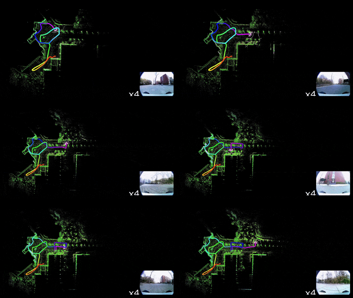
Generally, there are two ways to solve the problem of Localization,
- Mapping then Localizing: Create a Map of the environment(mapping) and later use that map to estimate the robot’s position (pose). Doing localization on a pre-built map is much efficient than SLAM.
- SLAM: Simultaneously creating the map and estimating the robot location in that map, as the robot moves. SLAM is computationally heavier than Mapping then Localizing.
From the perspective of a robust solution, SLAM sounds more effective because creating a new map every time confronted with an unknown surrounding is inefficient.
NB:
- Pose precisely means 6 Degrees of Freedom(DoF) [x, y, z, r, p, y], here x,y,z are the Cartesian coordinates, r, p, y are Euler angles in the case of 3D space.
- We have used the terms camera pose and robot pose interchangeably; both mean location of the robot in a 3D coordinate frame.
What is Visual SLAM?
When we use a camera as input for a SLAM algorithm, it’s called Visual SLAM. If a single camera is used, it’s known as Monocular Visual SLAM. When two or an array of cameras are involved, it’s referred to as Stereo Visual SLAM.
Let’s briefly describe some of the main advantages and disadvantages of stereo and monocular visual SLAM. Note that this post will concentrate on monocular for now, but we might document and post about stereo SLAM implementation later in the series.
| Aspect | Stereo SLAM | Mono Visual SLAM |
| Trajectory Estimation | Pro: Can estimate the exact trajectory in meters | Con: Estimates trajectory unique up to a scale factor |
| Robustness | Pro: Generally more robust due to more data | Con: May be less robust due to fewer data points |
| Computational Complexity | Con: Higher computational requirements | Pro: Lower computational requirements |
| 3D Mapping Capabilities | Con: Requires two cameras and calibration | Pro: Requires only one camera, simpler setup |
| 3D Reconstruction Detail | Pro: Produces accurate and dense 3D maps | Con: Produces less accurate and sparser 3D maps |
| Environmental Adaptability | Pro: Better at capturing fine details and depth information | Con: Struggles with fine details and depth accuracy |
| Setup Complexity | Con: Can be affected by lighting differences between cameras | Pro: Consistent performance with single camera setup |
What is Monocular SLAM?
Problem Formulation
We have intuitively understood Monocular Visual SLAM. Let’s now understand how it is formulated mathematically.
Input:
Given a sequence of camera frames of the environment from time ![]() , to
, to ![]() , represented as,
, represented as, ![]()
Output:
Find, the trajectory of the camera (robot) ![]() , here,
, here, ![]() is the camera’s pose.
is the camera’s pose.
And the map of the environment ![]() , pt represents the 3D coordinates.
, pt represents the 3D coordinates.
Objective:
Given the visual observations, maximize the probability (posterior) of the trajectory X and map M. Posterior probability is described as the probability of an event, given the observed data. Sounds familiar? It’s the left-hand of Bayes’ theorem.
![]()
Monocular Visual SLAM is divided into smaller problems, Mapping and Odometry.
Here,
- Mapping or
 : This is the probability (posterior) of map
  , given the trajectory
  and Camera frame
  .
. - Odometry or
 : This is the probability (posterior) of camera (robot) trajectory
  , given visual data
  .
.
Monocular Visual SLAM Algorithm Outline: How Monocular SLAM Works?
Let’s, understand how Monocular SLAM works. To begin with, algorithms involved in Monocular Visual SLAM can be divided into two main groups of algorithms Front-end and Back-end Algorithms.
- Front-end Algorithms: Algorithms responsible for estimating the camera pose and 3D map points.
- Back-end Algorithms: Algorithms responsible to optimize the estimated camera pose and mapping.
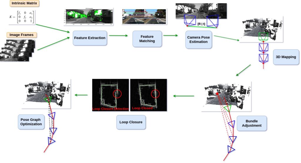
First the camera captures two images, ![]() and
and ![]() . Then these images are Undistort. After that below frontend algorithms are applied to estimate the camera pose and 3D map, and then we use the Back-end algorithms to optimize the previously estimated poses and map points. Let’s understnad how its done,
. Then these images are Undistort. After that below frontend algorithms are applied to estimate the camera pose and 3D map, and then we use the Back-end algorithms to optimize the previously estimated poses and map points. Let’s understnad how its done,
Front-end Algorithms:
- Feature Extraction: After the images
 and
and  are captured, we perform feature extraction on both the images. Say,
  and
and  are the features extracted from image
  and
and  respectively.
 - Feature Matching: Next we find the feature correspondences between the extracted feature points in
 and
and  . This feature matching can also be done by tracking the features from image
  to
to  .
. - Pose Estimation: Compute the relative camera pose between frames using tracked or matched feature points via epipolar geometry. Epipolar geometry takes the corresponding points from
 ,
,  and the camera intrinsic matrix.
 - Triangulation: Using the relative camera pose and the corresponding points we perform Triangulation to estimate the 3D coordinates of the surroundings.
- Local Mapping: As the camera moves, the estimated 3D points are accumulated over time. Which turns into a Local Map of the surrounding where the camera moved.
Now that, the initial camera pose and 3D map point estimations are done, we use the back-end algorithms to optimize them.
Back-end Algorithms:
- Bundle Adjustment: Bundle Adjustment refines the camera poses and 3D points by minimizing the reprojection error across all observations.
- Loop Closure Detection: There are times when the camera visits same place twice. In those situations we Identify the previously visited locations using methods like bag-of-words or place recognition techniques. The loop closing detection information later send to Pose Graph optimization.
- Pose Graph Optimization: When a loop is detected, we use Pose Graph optimization, to adjust the entire trajectory and map, which helps to maintain global consistency.
Don’t worry if you don’t understand all the steps mentioned above. Each point will be explained in great detail and in simple, layman’s terms in the text to follow.
Front-end Algorithms
Feature Extraction
Features are digital expression of image information. A good set of features is crucial to the final performance on the specified task, so researchers have done comprehensive work on extracting features for many years.
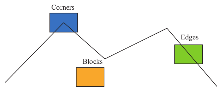
These features in classical computer vision are different from the deep learning features. In classical computer vision these features are handcrafted and represented as feature points, feature points are some special places in the image. Taking Figure 1 as an example, we can see the corners, edges, and blocks as representative places in the image.
A feature point is composed of two parts: key point and descriptor.
- key point: The key point refers to the 2D position(on image) of the feature point. Some types of key points also hold other information, such as the orientation and size.
- descriptor: The descriptor is usually a vector, describing the information of the pixels around the key point. Descriptors should be designed such that features with similar appearances have similar descriptors. Thus, if two feature descriptors are close in vector space, they can be considered the same feature.
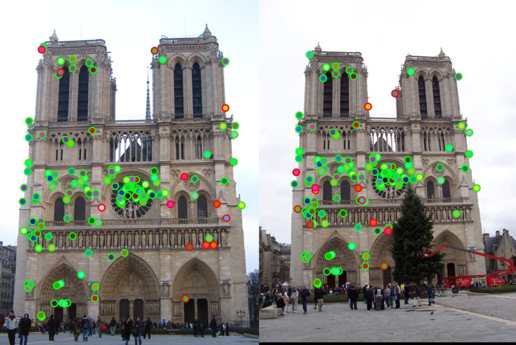
SIFT (Scale-Invariant Feature Transform) is one of the well known classic feature extraction algorithms, known for its accuracy and robustness. Contrary to that, SIFT has a good amount of calculations, which makes it computationally heavy. ORB (Oriented FAST and Rotated BRIEF) feature on the other hand is widely used for real-time feature extraction. It uses a modified version of FAST (Oriented FAST) with the extremely fast binary descriptor BRIEF, significantly accelerating the entire image feature extraction process.
Code:
Below is the OpenCV python code for feature extraction using ORB.
# Initialize the ORB detector with 5k keypoints
orb = cv2.ORB_create(nfeatures=5000)

# Detect keypoints and compute descriptors
keypoints, descriptors = orb.detectAndCompute(image, None)
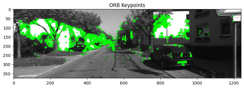
ORB Feature Extraction Explained:
Main idea of ORB Feature extraction is, if a pixel is very different from the neighbour pixels (too bright or too dark), it is more likely to be a corner point. Its entire procedure is as follows,
- Select pixel
 in the image assuming its brightness as
  .
. - Set a threshold
 (for example, 20% of
  ).
). - Take the pixel
 as the centre, and select the 16 pixels on a circle with a radius of 3.
 - If there are consecutive
 points on the selected circle whose brightness is greater than
  or less than
  , then the central pixel p can be considered a feature point. Value of
  is usually 12, 11 or 9.
 - Iterate through the above four steps on each pixel.
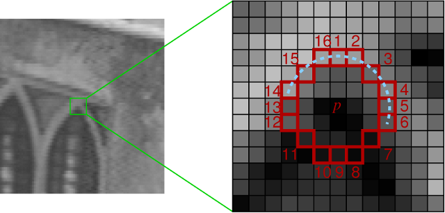
A trick is used to reject most non-corner points by first examining the pixels at positions 1, 9, 5, and 13. At least N of these pixels must have a brightness greater than ![]() or less than
or less than ![]() for the point to be considered a corner.
for the point to be considered a corner.
Right now, you might not understand how it relates to Monocular SLAM, but bear with me. As you follow the sections, you will be able to connect the dots.
Feature Matching
Feature Matching follows Feature Extraction. Feature Matching is an important part in Visual SLAM, used to find the matched features between two consecutive frames.
In computer vision terms, it means finding feature correspondences within the 2 images. Say, you have ![]() features from
features from ![]() th frame, and
th frame, and ![]() corresponding features from frame
corresponding features from frame ![]() .
.
For each point in frame I, compute the sum of squared differences (SSD) with all points in ![]() . Calculate the ratio of the best match (lowest distance) to the second-best match (second lowest distance). Keep the matched pair if this ratio is below a threshold, and reject it otherwise. This process filters confident feature correspondences, which are then used to estimate the camera’s rotation and translation in the world coordinate frame.
. Calculate the ratio of the best match (lowest distance) to the second-best match (second lowest distance). Keep the matched pair if this ratio is below a threshold, and reject it otherwise. This process filters confident feature correspondences, which are then used to estimate the camera’s rotation and translation in the world coordinate frame.
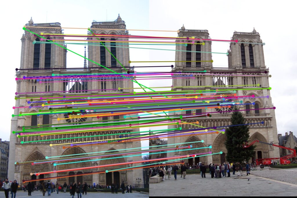
This code initializes an ORB detector to find keypoints and compute descriptors for two images, matches the descriptors using cv2.BFMatcher(), and sorts the matches by distance to identify the best matches.
Code:
# Initialize the ORB detector
orb = cv2.ORB_create(nfeatures=1000)

# Detect keypoints and compute descriptors for the first image
keypoints1, descriptors1 = orb.detectAndCompute(image1, None)

# Detect keypoints and compute descriptors for the second image
keypoints2, descriptors2 = orb.detectAndCompute(image2, None)

# Initialize the BFMatcher with default params
bf = cv2.BFMatcher(cv2.NORM_HAMMING, crossCheck=True)

# Match descriptors between frame I and frame I+1
matches = bf.match(descriptors1, descriptors2)

# Sort matches by distance (best matches first)
matches = sorted(matches, key=lambda x: x.distance)

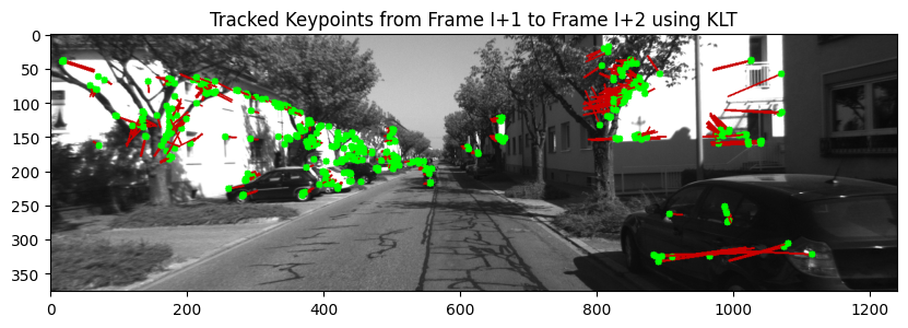
Feature tracking can be used to replace feature matching, for the task of following keypoints from frame to frame. Tracking keypoints is computationally efficient, which is crucial for real-time applications. But, there are cases where tracking can fail, such as, Large Motion, Drift from Error Accumulation and Missing Correspondences.
Below is the code for tracking feature points from frame I to frame ![]() . In
. In cv2.calcOpticalFlowPyrLK function we are passing frame ![]() ,
, ![]() and feature points from the
and feature points from the ![]() frame.
frame.
Code:
# Parameters for lucas kanade optical flow
lk_params = dict(winSize=(15, 15),

maxLevel=2,
criteria=(cv2.TERM_CRITERIA_EPS |   cv2.TERM_CRITERIA_COUNT, 10, 0.03))

# Calculate optical flow
points2, status, err = cv2.calcOpticalFlowPyrLK(image1, image2, points1, None, **lk_params)

# Select good points
good_new = points2[status.ravel() == 1]
good_old = points1[status.ravel() == 1]
Pose Estimation
Camera Pose Estimation is very important because you can estimate the 3D map only after you do that. Pose estimation is mathematically intensive. To grasp this topic, we first need to learn the basics and become familiar with common terms.
To begin with, let’s understand the world, camera, and image coordinate frame, how we capture a 3D object in a 2D image (Image formation), Epipolar Geometry.
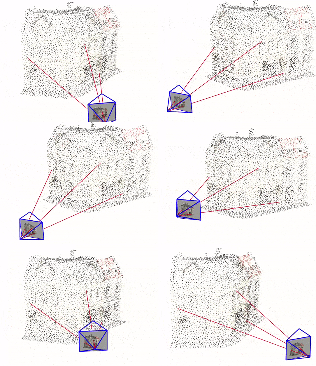
You can click here to experience an interactive version of this visualization
World Coordinates Frame
The World Coordinates Frame(WCF) is a global reference frame used in computer vision, robotics, and 3D graphics to define the positions and orientations of objects in a scene. You can consider any 3D location in the environment as the origin of the WCF. For Example, a robot supposed to operate at a University Campus can assume the College Gate as the WCF.
Camera Coordinate Frame
Say you have a camera somewhere in a World Coordinate frame. Now, if you consider the location of the camera as the origin and reference the location of any object wrt that camera location, then the coordinate frame will be called as Camera Coordinate Frame.
The relationship between the camera and world coordinate frames (3D to 3D), defined by some parameters represented as Extrinsic Matrix ![]() . This matrix helps in coordinate transformation from world to camera coordinate or vice versa.
. This matrix helps in coordinate transformation from world to camera coordinate or vice versa.
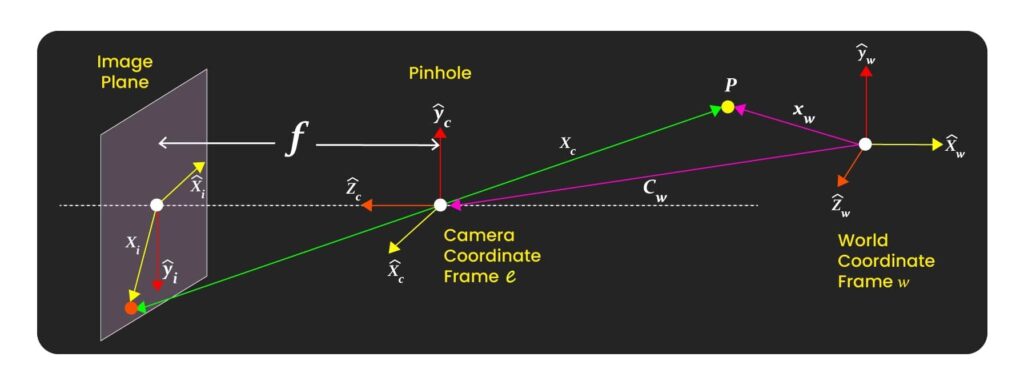
Image Coordinate Frame
Image Coordinate Frame is the coordinate of the image. This is in 2D. A Prospective project is used for this 3D to 2D transformation. Image coordinate frame can be related to the camera coordinate frame through the intrinsic camera parameters also known as Intrinsic Matrix (K).
If all this matrix and coordinate stuff is still Greek to you, just understand that a camera has two Matrices: the Extrinsic Matrix and the Intrinsic Matrix. First, a 3D object from the World Frame is brought to the Camera Frame(3D to 3D) using the Extrinsic Matrix, and then Intrinsic Matrix is used to bring the object from the Camera Frame to the image plane/frame (3D to 2D).
Later parts will help you to understand this topic in greater detail.
Image Formation Explained
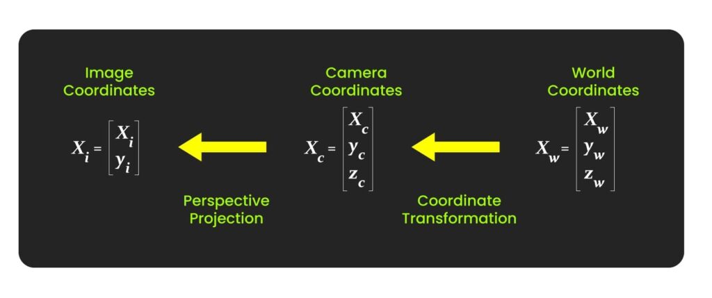
When we capture an image, the 3D points of the object are transformed and brought to the camera coordinate. This is a 3D to 3D transformation; this is done using an extrinsic matrix. Mathematically its represented as,
![]()
Here,
 = Rotation Matrix a matrix representing rotation (or roll, pitch, yaw) in a 3D coordinate system (3×3)
 = Translation Matrix
  in a 3D coordinate system (3×1)
 = 3D Coordinates in the World Coordinate Frame
 = 3D Coordinates in the Camera Coordinate Frame
 = Extrinsic Matrix (4×4)
NB: ![]() and
and ![]() , represent the rotation and translation of the camera coordinate frame wrt the World Coordinate Frame.
, represent the rotation and translation of the camera coordinate frame wrt the World Coordinate Frame.
Now that the object is represented in the camera Coordinate Frame, we use the Intrinsic matrix, ![]() , to transform the object point in 3D to the object point in 2D. Through this transformation, the object in the camera coordinate frame is projected to the image plane.
, to transform the object point in 3D to the object point in 2D. Through this transformation, the object in the camera coordinate frame is projected to the image plane.
![]()
Here,
 = Intrinsic Matrix (3×1)
 = 2D coordinates in image plane
 = 3D Coordinates in the Camera Coordinate Frame
Epipolar Geometry Explained
When the camera is monocular, we only know the 2D pixel coordinates, so the problem is to estimate the motion according to two sets of 2D points. This problem is solved by epipolar geometry.
You might wonder, if epipolar geometry is typically taught in a stereo vision class, why are we discussing it in a Monocular SLAM context? Well, it’s because you can’t estimate depth from just a single image. To estimate depth, you need more than one image. When multiple images come into play, we use epipolar geometry to figure out depth. In Monocular SLAM, we use image frames from different timestamps to estimate depth, making epipolar geometry super important.
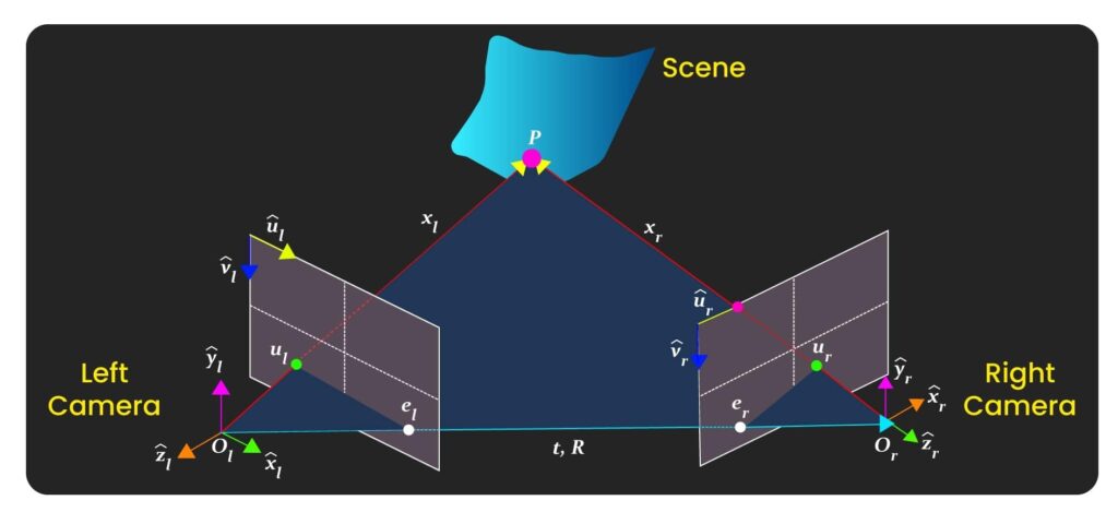
Epipolar geometry describes the relationship between two camera views of the same 3D scene. The epipolar plane is defined by the optical centers of the two cameras ![]() and
and ![]() and a 3D point
and a 3D point ![]() , intersection of the epipolar plane and image frames represents the epipolar lines
, intersection of the epipolar plane and image frames represents the epipolar lines ![]() and
and ![]() . These lines indicate where corresponding points must lie, reducing the search for matches from 2D to 1D. The epipoles
. These lines indicate where corresponding points must lie, reducing the search for matches from 2D to 1D. The epipoles ![]() and
and ![]() are where the baseline (the line joining
are where the baseline (the line joining ![]() and
and ![]() ) intersects the image planes. To determine the motion between frames
) intersects the image planes. To determine the motion between frames ![]() and
and ![]() , defined by rotation
, defined by rotation ![]() and translation
and translation ![]() , feature points
, feature points ![]() in
in ![]() and
and ![]() in
in ![]() must correspond correctly, projecting the same 3D point
must correspond correctly, projecting the same 3D point ![]() . The fundamental matrix
. The fundamental matrix ![]() , encapsulates this relationship, aiding in correspondence and 3D reconstruction tasks.
, encapsulates this relationship, aiding in correspondence and 3D reconstruction tasks.
Before proceeding further, let’s understand a few important equations from Epipolar Geometry. To understand how they are derived, please watch these videos mentioned at the Learning Material Section(bottom).
 (3D to 3D transformation)
 (Epipolar Constraint in 3D)
 (Essential matrix)
 (perspective projection equation)
 (perspective projection equation)
 (Relation between
  and
and  )
) (Epipolar Constraint in 2D)
Here,
 = Point in left camera’s coordinate system
 = Point in right camera’s coordinate system
 = Rotation matrix from right to left camera
 = Translation vector from right to left camera
 = Essential matrix
 = x-coordinate in pixel space of the left camera image
 = y-coordinate in pixel space of the left camera image
 = Focal length of the camera in x-direction
 = Focal length of the camera in y-direction
 = Homogeneous coordinates of a point in the left image
 = Homogeneous coordinates of a point in the right image
 = Depth (z-coordinate) in the left camera’s coordinate system
 = x-coordinate of the optical centre in the image
 = y-coordinate of the optical centre in the image
 = Intrinsic matrix of the left camera
 = Intrinsic matrix of the right camera
 = Fundamental matrix
Given a small subset(8 points only) of correspondences (generated points from step 1 and 2), we solve for ![]() , to find the fundamental matrix
, to find the fundamental matrix ![]() . In a matrix form it looks like this,
. In a matrix form it looks like this,
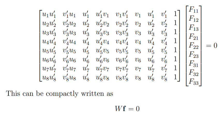
Here, ![]() is an
is an ![]() × 9 matrix derived from
× 9 matrix derived from ![]() ≥ 8 correspondences and f is the value of the Fundamental matrix we desire.
≥ 8 correspondences and f is the value of the Fundamental matrix we desire.
This system of equations from above, can be answered by solving the linear least squares by Singular Value Decomposition (SVD). After we find the value of ![]() , we can use this in the 6th equation to calculate the value of
, we can use this in the 6th equation to calculate the value of ![]() . Later, SVD can be used on
. Later, SVD can be used on ![]() to estimate
to estimate ![]() .
.
This code extracts the matched key-points from two images, sets up the camera’s intrinsic parameters, and then computes the Fundamental matrix using the RANSAC (Random sample consensus) method to robustly estimate which matches are inliers.
Code:
# Extract matched keypoints
pts1 = np.float32([keypoints1[m.queryIdx].pt for m in matches])
pts2 = np.float32([keypoints2[m.trainIdx].pt for m in matches])

# Camera intrinsic parameters (example values, replace with your camera's calibration data)
K = np.array([[fx, 0, cx],
              [0, fy, cy],
              [0, 0, 1]])

# Compute the Fundamental matrix using RANSAC
F, inliers = cv2.findFundamentalMat(pts1, pts2, cv2.FM_RANSAC)

# Compute the Essential matrix using the camera's intrinsic parameters
E = K.T @ F @ K

# Decompose the Essential matrix to get R and t
_, R, t, mask = cv2.recoverPose(E, pts1_inliers, pts2_inliers, K)
In real-world scenarios, feature matching often includes outliers (erroneous correspondences) due to incorrect correspondences, noise, or occlusions. RANSAC helps identify and exclude these outliers to compute a more accurate Essential Matrix. After estimating the value of the Essential Matrix, we can use SVD to decompose it to R and t as mentioned in the 3rd equation.
Triangulation
In the previous step, we introduced using the epipolar constraint to estimate the camera motion and discussed its limitations. After estimating the motion, the next step is to use the camera motion to estimate the spatial positions of the feature points. In monocular SLAM, the depths of the pixels cannot be obtained by a single image. We need to estimate the depths of the map points by the method of triangulation.
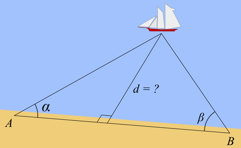
Triangulation is a popular method, used for determining the geographic location of a point in old times. Triangulation used in epipolar geometry and triangulation for geolocation relies on similar concepts, such as,
- Both methods use the principle of triangulation to determine unknown positions based on known reference points and measurements.
- Both involve geometric calculations to find the intersection of lines or rays in space.
The triangulation used in epipolar geometry differs in that, it relies on image correspondences and camera calibration parameters.
To solve for estimating the 3D point of an object, triangulation is used as follows,
Let (![]() ,
, ![]() ) be the coordinates of a point in the first image, and (
) be the coordinates of a point in the first image, and (![]() ,
, ![]() ) be the coordinates of the corresponding point in the second image. Construct the projection matrix (
) be the coordinates of the corresponding point in the second image. Construct the projection matrix (![]() ) for both camera pose at time
) for both camera pose at time ![]() and
and ![]() .
.
![]()
The relationship between a 3D point ![]() and its 2D projection
and its 2D projection ![]() in an image is given by the camera projection matrix P:
in an image is given by the camera projection matrix P:
![]()
we have two projection matrices ![]() and
and ![]() ,
, ![]() ,
, ![]() . Here,
. Here, ![]() and
and ![]() are
are ![]() matrices that combine the intrinsic and extrinsic parameters of the cameras. The cross product
matrices that combine the intrinsic and extrinsic parameters of the cameras. The cross product ![]() of two vectors
of two vectors ![]() and
and ![]() results in a vector orthogonal to both, implying:
results in a vector orthogonal to both, implying:
![]()
![]()
These equations arise because the cross product of a point with its projection must be zero if the point indeed lies on the projected line. After expanding the Cross Product we get,

Here, A is a matrix constructed from the components of ![]() ,
, ![]() ,
, ![]() , and
, and ![]() . The solution to this homogeneous system is typically found using linear least squares, often via Singular Value Decomposition (SVD), to find the best estimate of
. The solution to this homogeneous system is typically found using linear least squares, often via Singular Value Decomposition (SVD), to find the best estimate of ![]() .
.
Code:
import numpy as np

def add_ones(pts):
    """Helper function to add a column of ones to a 2D array (homogeneous coordinates)."""
    return np.hstack([pts, np.ones((pts.shape[0], 1))])

def triangulate(pose1, pose2, pts1, pts2):
    # Initialize the result array to store the homogeneous coordinates of the 3D points
    ret = np.zeros((pts1.shape[0], 4))

    # Invert the camera poses to get the projection matrices
    pose1 = np.linalg.inv(pose1)
    pose2 = np.linalg.inv(pose2)

    # Loop through each pair of corresponding points
    for i, p in enumerate(zip(add_ones(pts1), add_ones(pts2))):
        # Initialize the matrix A to hold the linear equations
        A = np.zeros((4, 4))

        # Populate the matrix A with the equations derived from the projection matrices and the points
        A[0] = p[0][0] * pose1[2] - pose1[0]
        A[1] = p[0][1] * pose1[2] - pose1[1]
        A[2] = p[1][0] * pose2[2] - pose2[0]
        A[3] = p[1][1] * pose2[2] - pose2[1]

        # Perform SVD on A
        _, _, vt = np.linalg.svd(A)

        # The solution is the last row of V transposed (V^T), corresponding to the smallest singular value
        ret[i] = vt[3]

    # Return the 3D points in homogeneous coordinates
    return ret
The inversion in 12th and 13th line is necessary because the poses given are typically transformations from the world coordinate frame to the camera coordinate frame, and we need the inverse to convert from camera to world coordinates.
The code for this is provided in the github repository, you can download and experiment.
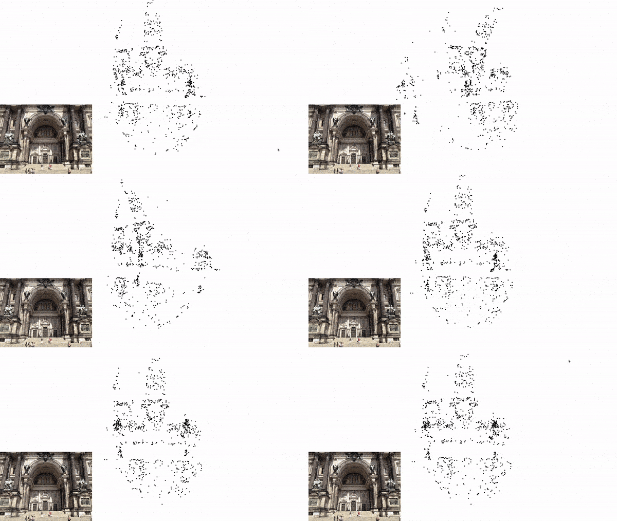
Local Mapping
Local Mapping in Visual SLAM involves updating the local map with new 3D points derived from recent observations. The newly triangulated points are added to the local map. Keyframes are selected to represent significant positions. Keyframes in Visual SLAM refer to both the image captured at a specific time and the corresponding camera pose (position and orientation) at that time. The difference between a Keyframe and a normal frame, is that Keyframes typically contain a high density of detected features (key points), which are used for mapping and pose estimation. Only a subset of all captured normal frames are selected as keyframes.
Back-end Algorithms
Bundle Adjustment
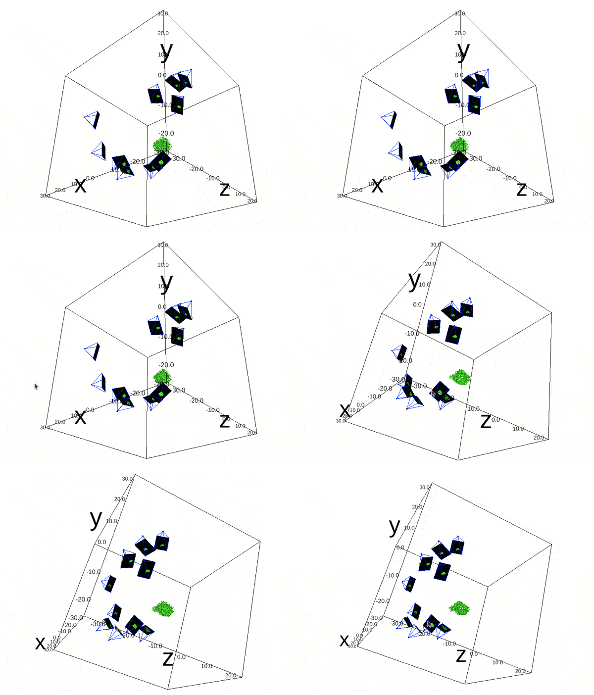
Bundle adjustment is a very simple concept that is widely used in the SLAM and Structure from motion (SfM) community. Bundle adjustment is a process used in 3D mapping to refine the positions of points in a scene and the positions and angles of the cameras that took pictures of those points.
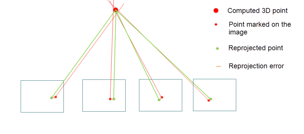
The process minimizes the difference between where points appear in the images and where they should appear based on the 3D model. This difference is called the reprojection error. Reducing this error helps create a precise 3D map and accurate camera positions.
Bundle adjustment is similar to gradient descent in that both are optimization techniques aimed at minimizing an error metric. In gradient descent, the algorithm iteratively adjusts parameters (such as weights in a neural network) to reduce the difference between predicted and actual values. Similarly, in bundle adjustment, the algorithm iteratively refines the 3D point coordinates and camera poses to minimize the re-projection error.
Code:
def vertex_to_points(optimizer, first_point_id, last_point_id):
    """ Converts g2o point vertices to their current 3d point estimates. """
    vertices_dict = optimizer.vertices()
    estimated_points = list()
    for idx in range(first_point_id, last_point_id):
        estimated_points.append(vertices_dict[idx].estimate())
    estimated_points = np.array(estimated_points)
    xs, ys, zs = estimated_points.T
    return xs, ys, zs

ipv.show()
for i in range(100):
    optimizer.optimize(1)
    xs, ys, zs = vertex_to_points(optimizer, first_point_id, last_point_id)
    scatter_plot.x = xs
    scatter_plot.y = ys
    scatter_plot.z = zs
    time.sleep(0.25)
Reprojection Error(RPE) can be expressed as a summation over all cameras and points
![]()
![]()
Here,
 : The total reprojection error, which we aim to minimize.
 : A camera from the set of all cameras C.
 : A 3D point from the set of all 3D points P.
 : The corresponding 2D point observed in the image captured by the camera c.
 : The distance between the observed 2D point
  and the projected 3D point p onto the image plane of the camera c using the projection function Q.
 : A binary variable that indicates whether the 3D point p is observed by the camera c. If
  , the point is observed; if
  , it is not.
# Function to compute reprojection error
def compute_reprojection_error(intrinsics, extrinsics, points_3d, observations):
    total_error = 0  # Initialize the total error to zero
    num_points = 0  # Initialize the number of points to zero

    # Iterate through each camera's extrinsics and corresponding 2D observations
    for (rotation, translation), obs in zip(extrinsics, observations):
        # Project the 3D points to 2D using the current camera's intrinsics and extrinsics
        projected_points = project_points(points_3d, intrinsics, rotation, translation)

        # Calculate the Euclidean distance (reprojection error) between the projected points and the observed points
        error = np.linalg.norm(projected_points - obs, axis=1)

        # Accumulate the total error
        total_error += np.sum(error)

        # Accumulate the total number of points
        num_points += len(points_3d)

    # Calculate the mean reprojection error
    mean_error = total_error / num_points

    return mean_error  # Return the mean reprojection error
Loop Closure Detection
Loop closure is one of the algorithms used in the backend. Loop closure detection allows the system to identify when the robot returns to a previously visited location, effectively closing the loop in its path. This ability is crucial for precise map construction and localization, as it helps reduce drift errors that build up over time.
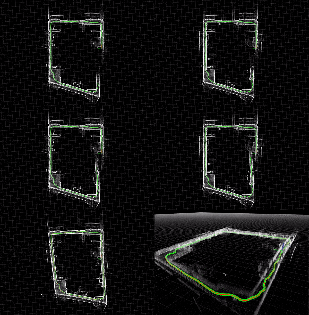
The SLAM system maintains a graph where nodes represent camera poses and edges represent spatial constraints. When a loop closure is detected, additional edges are added to the graph to represent the newly recognized connections, and optimization techniques like pose graph optimization or bundle adjustment are applied to minimize the overall error.
Bag-of-Words (BoW) is a place recognition algorithm used in loop closure detection for Visual SLAM. It converts image features into a vector of visual words, creating a compact descriptor. During loop closure detection, the current image’s BoW descriptor is compared with those from previously visited locations. Similarities between descriptors indicate revisited locations, enabling the system to detect loop closures efficiently and accurately, even in large environments.
DBoW2 is an open source C++ library for indexing and converting images into a bag-of-word representation. This library is also used in ORB-SLAM.
Pose Graph Optimization
Pose Graph Optimization is a crucial back-end step in Visual SLAM used to refine the estimated poses of the camera (or robot) over time to ensure global consistency in the map. This optimization is essential because, during the mapping process, small errors in pose estimation can accumulate, leading to significant drift. Pose graph optimization helps correct these errors by simultaneously optimizing the entire trajectory of poses.
When loop closures are detected, pose graph optimization integrates these constraints to adjust the poses and reduce drift.
Difference between Pose Graph Optimization and Bundle Adjustment: Pose Graph Optimization might sound the same as Bundle Adjustment, but Bundle adjustment aims to refine both the 3D point coordinates and the camera poses simultaneously. The goal is to minimize the reprojection error. On the contrary, Pose Graph Optimization is only for camera pose refinement.
Simple Monocular Visual SLAM in Python OpenCV
There are few Python implementations available on the Internet because they are inefficient and not real-time. But from an educational point of view, Python implementations are important, as they are a good starting point for anyone who is starting out with SLAM.
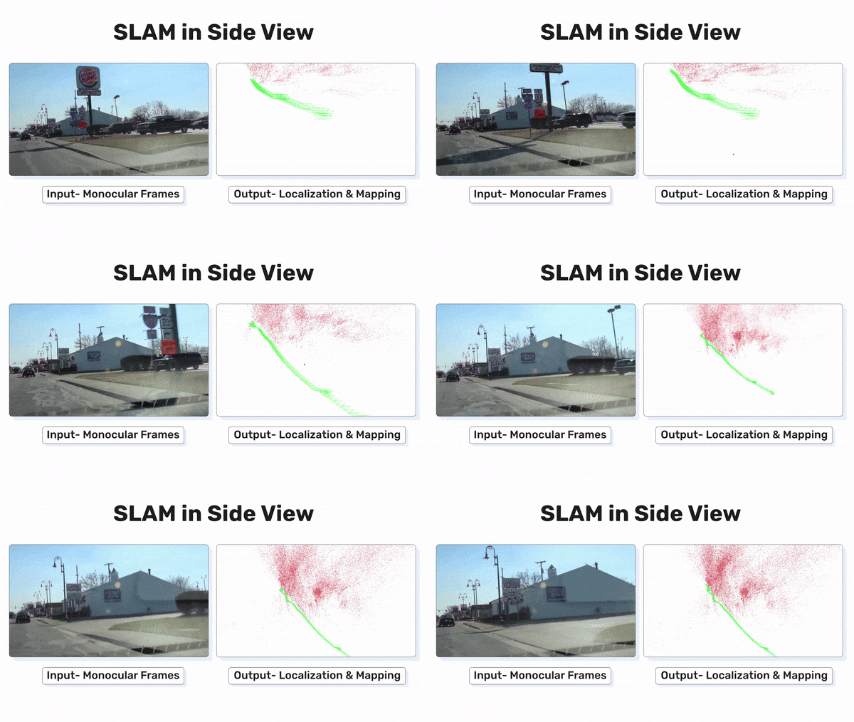
For this reason, we will be going through a simple implementation of Monocular Visual SLAM in Python consisting of only 4 files. This implementation mostly covers the front-end of the Visual SLAM, which is camera pose estimation and 3D mapping. Above Figure 1(d) is the output of this python implementation.
Looks cool! Let’s understand how it’s implemented.
The code is structured as below, consisting of only 4 files and one test video. This is not the most accurate implementation of monocular visual SLAM but it produces decent results. Let’s go through the file structure.
├── display.py
├── extractor.py
├── main.py
├── pointmap.py
└── test_countryroad.mp4
- extractor.py: This file contains code for all the utilities used to estimate the camera pose, such as,
- Feature extraction
extract - Feature matching
match_frames - Camera pose estimation:
extractPose - Coordinate normalization and de-normalization:
normalizeanddenormalize - Class to define keyframe:
Frame
- Feature extraction
- display.py: This file contains the code for image visualization using the library called Simple DirectMedia Layer(SDL2).
- pointmap.py: This file contains the code for 3D point and Map visualization using pangolin.
- main.py: This file takes a video file and its intrinsic matrix, and calls functions from other files for 3D mapping and camera pose estimation.
NB: We have explained all the classes and functions after a block of code. But, please follow the comments in the code section as well. It’s better explained there.
Explanation of main.py
Let’s go through all of them one by one. We will start with the main.py.
import cv2
from display import Display
from extractor import Frame, denormalize, match_frames, IRt, add_ones
import numpy as np
from pointmap import Map, Point

### Camera intrinsics
# define principal point offset or optical center coordinates
W, H = 1920//2, 1080//2

# define focus length
F = 270

# define intrinsic matrix and inverse of that
K = np.array(([F, 0, W//2], [0,F,H//2], [0, 0, 1]))
Kinv = np.linalg.inv(K)

# image display initialization
display = Display(W, H)

# initialize a map
mapp = Map()
mapp.create_viewer()
After the imports we, define a few very important parameters that are going to be used extensively throughout the code, that includes,
- optical centre coordinates
- focus length
- intrinsic matrix (and also the inverse)
- 3D Map, image display initialization
def process_frame(img):
    img = cv2.resize(img, (W, H))
    frame = Frame(mapp, img, K)
    if frame.id == 0:
        return

    # previous frame f2 to the current frame f1.
    f1 = mapp.frames[-1]
    f2 = mapp.frames[-2]

    idx1, idx2, Rt = match_frames(f1, f2)

    # X_f1 = E * X_f2, f2 is in world coordinate frame, multiplying that with
    # Rt transforms the f2 pose wrt the f1 coordinate frame
    f1.pose = np.dot(Rt, f2.pose)


    # The output is a matrix where each row is a 3D point in homogeneous coordinates [𝑋, 𝑌, 𝑍, 𝑊]
    # returns an array of size (n, 4), n = feature points
    pts4d = triangulate(f1.pose, f2.pose, f1.pts[idx1], f2.pts[idx2])


    # The homogeneous coordinates [𝑋, 𝑌, 𝑍, 𝑊] are converted to Euclidean coordinates
    pts4d /= pts4d[:, 3:]


    # Reject points without enough "Parallax" and points behind the camera
    # returns, A boolean array indicating which points satisfy both criteria.
    good_pts4d = (np.abs(pts4d[:, 3]) > 0.005) & (pts4d[:, 2] > 0)

    for i, p in enumerate(pts4d):
        # If the point is not good (i.e., good_pts4d[i] is False),
        # the loop skips the current iteration and moves to the next point.
        if not good_pts4d[i]:
            continue
        pt = Point(mapp, p)
        pt.add_observation(f1, i)
        pt.add_observation(f2, i)

    for pt1, pt2 in zip(f1.pts[idx1], f2.pts[idx2]):
        u1, v1 = denormalize(K, pt1)
        u2, v2 = denormalize(K, pt2)

        cv2.circle(img, (u1,v1), 3, (0,255,0))
        cv2.line(img, (u1,v1), (u2, v2), (255,0,0))

    # 2-D display
    display.paint(img)

    # 3-D display
    mapp.display()

if __name__== "__main__":
    cap = cv2.VideoCapture("/path/to/car.mp4")

    while cap.isOpened():
        ret, frame = cap.read()
        if ret == True:
            process_frame(frame)
        else:
            break
triangulate function is already discussed in the triangulation section.
This is the working of process_frame:
if frame.id == 0: returnis very important, because using a single frame we can’t estimate anything.- define the current and previous frame.
match_framesdoes feature matching, and finds correspondences in the current frame.- Rt transforms the f2 pose wrt the f1 coordinate frame.
triangulateestimated the 3d map points.- The homogeneous coordinates to Euclidean coordinates, by dividing each point W.
- Reject points without enough “Parallax” and points behind the camera.
- If the point follows the above condition we add that point to the map.
- After denormalizing all the good points, we draw the feature points(circle) and its tracking trails(line).
- After that we display the image and 3d map with camera pose estimation.
After, if __name__== "__main__": we are reading the video and sending the frames to `process_frame` function. If you have a specific video in mind, you can put its path here.
Explanation of extractor.py
Curious how function match_frames, denormalize are defined? Let’s go through extractor.py,
import cv2
import numpy as np
from skimage.measure import ransac
from skimage.transform import FundamentalMatrixTransform
import g2o

def add_ones(x):
    # creates homogenious coordinates given the point x
    return np.concatenate([x, np.ones((x.shape[0], 1))], axis=1)


def extractPose(F):
    # Define the W matrix used for computing the rotation matrix
    W = np.mat([[0, -1, 0], [1, 0, 0], [0, 0, 1]])

    # Perform Singular Value Decomposition (SVD) on the Fundamental matrix F
    U, d, Vt = np.linalg.svd(F)
    assert np.linalg.det(U) > 0

    # Correct Vt if its determinant is negative to ensure it's a proper rotation matrix
    if np.linalg.det(Vt) < 0:
        Vt *= -1

    # Compute the initial rotation matrix R using U, W, and Vt
    R = np.dot(np.dot(U, W), Vt)

    # Check the diagonal sum of R to ensure it's a proper rotation matrix
    # If not, recompute R using the transpose of W
    if np.sum(R.diagonal()) < 0:
        R = np.dot(np.dot(U, W.T), Vt)

    # Extract the translation vector t from the third column of U
    t = U[:, 2]

    # Initialize a 4x4 identity matrix to store the pose
    ret = np.eye(4)

    # Set the top-left 3x3 submatrix to the rotation matrix R
    ret[:3, :3] = R

    # Set the top-right 3x1 submatrix to the translation vector t
    ret[:3, 3] = t

    print(d)

    # Return the 4x4 homogeneous transformation matrix representing the pose
    return ret
add_onescreates homogenious coordinates given the point .
.- The
extractPosefunction computes the homogeneous transformation matrix representing the relative camera pose (rotation and translation) from a given Fundamental matrix
  using Singular Value Decomposition (SVD).
def extract(img):
    orb = cv2.ORB_create()

    # Detection
    pts = cv2.goodFeaturesToTrack(np.mean(img, axis=-1).astype(np.uint8), 1000, qualityLevel=0.01, minDistance=10)

    # Extraction
    kps = [cv2.KeyPoint(f[0][0], f[0][1], 20) for f in pts]
    kps, des = orb.compute(img, kps)

    return np.array([(kp.pt[0], kp.pt[1]) for kp in kps]), des
- The
extractfunction detects keypoints in an image using thecv2.goodFeaturesToTrack()method, converts them to ORB keypoints, and then computes ORB descriptors for these keypoints, returning their coordinates and descriptors.
def normalize(Kinv, pts):
    # The inverse camera intrinsic matrix 𝐾^(−1) transforms 2D homogeneous points
    # from pixel coordinates to normalized image coordinates.
    return np.dot(Kinv, add_ones(pts).T).T[:, 0:2]
- In
normalizefunction, the inverse camera intrinsic matrix 𝐾 − 1 transforms 2D homogeneous points from pixel coordinates to normalized image coordinates. This transformation centres the points based on the principal point (𝑐𝑥 , 𝑐𝑦) and scales them according to the focal lengths 𝑓𝑥 and 𝑓𝑦, effectively mapping the points to a normalized coordinate system where the principal point becomes the origin and the distances are scaled by the focal lengths.
def denormalize(K, pt):
    # Converts a normalized point to pixel coordinates by applying the
    # intrinsic camera matrix and normalizing the result.
    ret = np.dot(K, [pt[0], pt[1], 1.0])
    ret /= ret[2]
    return int(round(ret[0])), int(round(ret[1]))
denormalizefunction converts a normalized point to pixel coordinates by applying the.
def match_frames(f1, f2):
    # The code performs k-nearest neighbors matching on feature descriptors
    bf = cv2.BFMatcher(cv2.NORM_HAMMING)
    matches = bf.knnMatch(f1.des, f2.des, k=2)

    # applies Lowe's ratio test to filter out good
    # matches based on a distance threshold.
    ret = []
    idx1, idx2 = [], []
    for m, n in matches:
        if m.distance < 0.75*n.distance:
            p1 = f1.pts[m.queryIdx]
            p2 = f2.pts[m.trainIdx]

            # Distance test
            # dditional distance test, ensuring that the
            # Euclidean distance between p1 and p2 is less than 0.1
            if np.linalg.norm((p1-p2)) < 0.1:
                # Keep idxs
                idx1.append(m.queryIdx)
                idx2.append(m.trainIdx)
                ret.append((p1, p2))
                pass


    assert len(ret) >= 8
    ret = np.array(ret)
    idx1 = np.array(idx1)
    idx2 = np.array(idx2)

    # Fit matrix
    model, inliers = ransac((ret[:, 0],
                            ret[:, 1]), FundamentalMatrixTransform,
                            min_samples=8, residual_threshold=0.005,
                            max_trials=200)

    # Ignore outliers
    ret = ret[inliers]
    Rt = extractPose(model.params)

    return idx1[inliers], idx2[inliers], Rt
- The
match_framesfunction matches ORB descriptors between two frames using BFMatcher with Lowe’s ratio test and additional distance test, filters inliers using RANSAC to fit a Fundamental matrix, and extracts the relative pose, returning the indices of inlier matches and the transformation matrix.
class Frame(object):

    def __init__(self, mapp, img, K):
        self.K = K  # Intrinsic camera matrix
        self.Kinv = np.linalg.inv(self.K)  # Inverse of the intrinsic camera matrix
        self.pose = IRt  # Initial pose of the frame (assuming IRt is predefined)

        self.id = len(mapp.frames)  # Unique ID for the frame based on the current number of frames in the map
        mapp.frames.append(self)  # Add this frame to the map's list of frames

        pts, self.des = extract(img)  # Extract feature points and descriptors from the image
        self.pts = normalize(self.Kinv, pts)  # Normalize the feature points using the inverse intrinsic matrix
Frameclass initializes a frame object with the intrinsic camera matrix, pose, and feature points and descriptors extracted from an image, and adds the frame to a map object.
Explanation of pointmap.py
Let’s, understand how pangolin is used for defining the map, and point class in the pointmap.py file,
from multiprocessing import Process, Queue
import numpy as np

import pangolin
import OpenGL.GL as gl

# Global map // 3D map visualization using pangolin
class Map(object):
    def __init__(self):
        self.frames = [] # camera frames [means camera pose]
        self.points = [] # 3D points of map
        self.state = None # variable to hold current state of the map and cam pose
        self.q = None # A queue for inter-process communication. | q for visualization process

    def create_viewer(self):
        # Parallel Execution: The main purpose of creating this process is to run
        # the `viewer_thread` method in parallel with the main program.
        # This allows the 3D viewer to update and render frames continuously
        # without blocking the main execution flow.

        self.q = Queue() # q is initialized as a Queue

        # initializes the Parallel process with the `viewer_thread` function
        # the arguments that the function takes is mentioned in the args var
        p = Process(target=self.viewer_thread, args=(self.q,))

        # daemon true means, exit when main program stops
        p.daemon = True

        # starts the process
        p.start()

    def viewer_thread(self, q):
        # `viewer_thread` takes the q as input
        # initializes the viz window
        self.viewer_init(1280, 720)
        # An infinite loop that continually refreshes the viewer
        while True:
            self.viewer_refresh(q)

    def viewer_init(self, w, h):
        pangolin.CreateWindowAndBind('Main', w, h)

        # This ensures that only the nearest objects are rendered,
        # creating a realistic representation of the scene with
        # correct occlusions.
        gl.glEnable(gl.GL_DEPTH_TEST)

        # Sets up the camera with a projection matrix and a model-view matrix
        self.scam = pangolin.OpenGlRenderState(
            # `ProjectionMatrix` The parameters specify the width and height of the viewport (w, h), the focal lengths in the x and y directions (420, 420), the principal point coordinates (w//2, h//2), and the near and far clipping planes (0.2, 10000). The focal lengths determine the field of view,
            # the principal point indicates the center of the projection, and the clipping planes define the range of distances from the camera within which objects are rendered, with objects closer than 0.2 units or farther than 10000 units being clipped out of the scene.
            pangolin.ProjectionMatrix(w, h, 420, 420, w//2, h//2, 0.2, 10000),
            # pangolin.ModelViewLookAt(0, -10, -8, 0, 0, 0, 0, -1, 0) sets up the camera view matrix, which defines the position and orientation of the camera in the 3D scene. The first three parameters (0, -10, -8) specify the position of the camera in the world coordinates, indicating that the camera is located at coordinates (0, -10, -8). The next three parameters (0, 0, 0)
            # define the point in space the camera is looking at, which is the origin in this case. The last three parameters (0, -1, 0) represent the up direction vector, indicating which direction is considered 'up' for the camera, here pointing along the negative y-axis. This setup effectively positions the camera 10 units down and 8 units back from the origin, looking towards the origin with the 'up' direction being downwards in the y-axis, which is unconventional and might be used to achieve a specific orientation or perspective in the rendered scene.
            pangolin.ModelViewLookAt(0, -10, -8, 0, 0, 0, 0, -1, 0))
        # Creates a handler for 3D interaction.
        self.handler = pangolin.Handler3D(self.scam)

        # Creates a display context.
        self.dcam = pangolin.CreateDisplay()
        # Sets the bounds of the display
        self.dcam.SetBounds(0.0, 1.0, 0.0, 1.0, -w/h)
        # assigns handler for mouse clicking and stuff, interactive
        self.dcam.SetHandler(self.handler)
        self.darr = None

    def viewer_refresh(self, q):
        # Checks if the current state is None or if the queue is not empty.
        if self.state is None or not q.empty():
            # Gets the latest state from the queue.
            self.state = q.get()

        # Clears the color and depth buffers.
        gl.glClear(gl.GL_COLOR_BUFFER_BIT | gl.GL_DEPTH_BUFFER_BIT)
        # Sets the clear color to white.
        gl.glClearColor(1.0, 1.0, 1.0, 1.0)
        # Activates the display context with the current camera settings.
        self.dcam.Activate(self.scam)

        # camera trajectory line and color setup
        gl.glLineWidth(1)
        gl.glColor3f(0.0, 1.0, 0.0)
        pangolin.DrawCameras(self.state[0])

        # 3d point cloud color setup
        gl.glPointSize(2)
        gl.glColor3f(1.0, 0.0, 0.0)
        pangolin.DrawPoints(self.state[1])

        # Finishes the current frame and swaps the buffers.
        pangolin.FinishFrame()


    def display(self):
        if self.q is None:
            return
        poses, pts = [], []
        for f in self.frames:
            # updating pose
            poses.append(f.pose)

        for p in self.points:
            # updating map points
            pts.append(p.pt)

        # updating queue
        self.q.put((np.array(poses), np.array(pts)))
- The
Mapclass manages and visualizes a 3D map using pangolin, with frames representing camera poses and points representing 3D map points. It runs a separate viewer thread to continuously update and render the 3D scene without blocking the main program, initializing a Pangolin window, and setting up the camera and display context for 3D interaction. Thedisplaymethod updates the queue with the current camera poses and map points, which are then rendered in the viewer thread to visualize the trajectory and 3D points.
class Point(object):
    # A Point is a 3-D point in the world
    # Each point is observed in multiple frames

    def __init__(self, mapp, loc):
        self.frames = []
        self.pt = loc
        self.idxs = []

        # assigns a unique ID to the point based on the current number of points in the map.
        self.id = len(mapp.points)
        # adds the point instance to the map’s list of points.
        mapp.points.append(self)

    def add_observation(self, frame, idx):
        # Frame is the frame class
        self.frames.append(frame)
        self.idxs.append(idx)
The Point class represents a 3D point in the world observed in multiple frames. It initializes with a location and unique ID, adds itself to the map’s list of points, and records observations with associated frames and feature indices.
Explanation of display.py
Finally, the last file. In the display.py we will go through the image display code is written which uses sdl2,
import sdl2
import sdl2.ext
import cv2

class Display(object):
    def __init__(self, W, H):
        sdl2.ext.init()
        self.window = sdl2.ext.Window("Tim Slam", size=(W, H))
        self.window.show()
        self.W, self.H = W, H

    def paint(self, img):
        img = cv2.resize(img, (self.W, self.H))
        # Retrieves a list of SDL2 events.
        events = sdl2.ext.get_events()
        for event in events:
            # Checks if the event type is SDL_QUIT (window close event).
            if event.type == sdl2.SDL_QUIT:
                exit(0)
        # Retrieves a 3D numpy array that represents the pixel data of the window's surface.
        surf = sdl2.ext.pixels3d(self.window.get_surface())
        # Updates the pixel data of the window's surface with the resized image.
        # img.swapaxes(0, 1) swaps the axes of the image array to match the expected format of the SDL surface.
        surf[:, :, 0:3] = img.swapaxes(0, 1)
        # Refreshes the window to display the updated surface.
        self.window.refresh()
- The
Displayclass initializes an SDL2 window for displaying images. It provides apaintmethod that resizes a given image to fit the window, updates the window’s pixel data with the resized image, and handles window events such as closing. The image’s pixel data is swapped to match the SDL surface format, and the window is refreshed to display the updated image.
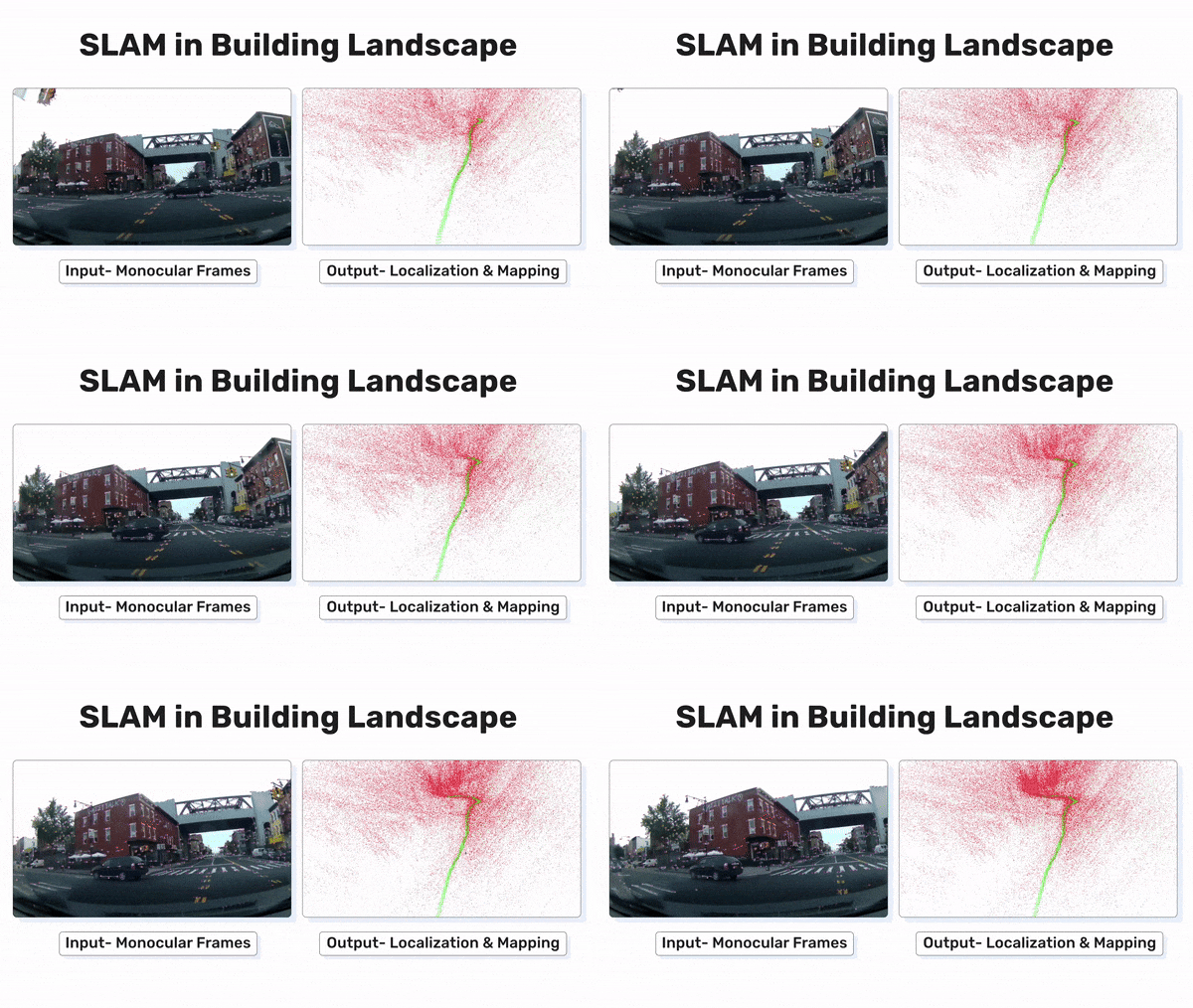
Gosh! this sure was a long post. We hope you understood the implementation and how all the steps connected with each other to perform simultaneous localization and mapping. We have added a few more resources at the bottom of this article, which has an end-to-end implementation of Monocular Visual SLAM in python, including all the backend algorithms, such as loop closure, pose graph optimization, bundle adjustment, using KDTree etc.
We are at the end of this article, and it’s a good time to learn about one of the breakthroughs in the field of monocular SLAM. Right now there are technologies like NeRF SLAM, Gaussian Splatting SLAM etc. but, knowing about the initial algorithm always gives you the whole perspective of the problem and the tools learned can be used elsewhere.
Overview of ORB-SLAM
ORB-SLAM was one of the breakthroughs in the field of visual SLAM. The unique thing about ORB-SLAM is that it has all the components that make a robust SLAM algorithm. The frontend and backend algorithms are efficiently planned, solely focusing on making the implementation more accurate at the same time, making it real-time. ORB-SLAM uses ORB for feature extraction, but all the SLAM that use ORB as feature extraction can’t be called ORB-SLAM. In the same way as described above, SLAM implementations use ORB as their feature extraction method, but the implementation can’t be called ORB-SLAM. Below are the contributions by ORB-SLAM,
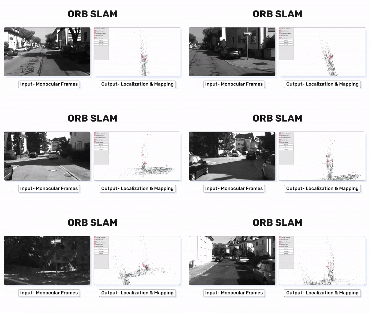
- Use of ORB Features for All Tasks: Utilizes the same ORB features for tracking, mapping, relocalization, and loop closing, ensuring efficiency, simplicity, and reliability.
- Real-Time Operation in Large Environments: Focuses tracking and mapping on a local covisible area using a covisibility graph, independent of the global map size.
- Real-Time Loop Closing: Optimizes a pose graph called the Essential Graph, built from a spanning tree, loop closure links, and strong edges from the covisibility graph.
- Real-Time Camera Relocalization: Provides significant invariance to viewpoint and illumination changes, allowing recovery from tracking failure and enhancing map reuse.
- Robust Initialization Procedure: Automatically and robustly initializes the map using model selection for both planar and non-planar scenes.
- Survival of the Fittest for Map Points and Keyframes: Adopts a policy of generous spawning but restrictive culling, improving tracking robustness and supporting lifelong operation by discarding redundant key-frames.
ORB-SLAM is an innovative approach to SLAM. But before that, multiple implementations similarly contributed to this field. Below is the time frame of each of them.

ORB-SLAM has two other extensions that were later released, ORB-SLAM 2 and ORB-SLAM 3.
- ORB-SLAM 2 supports the creation and management of multiple maps, and extends the original capabilities to handle both RGB-D and monocular cameras, allowing for efficient mapping and relocalization in diverse environments.
- ORB-SLAM 3 integrates inertial measurements (IMU) with visual data to enhance robustness and accuracy, and supports stereo and stereo-inertial camera systems, providing more versatility and precision in 3D mapping and localization tasks.
We will be going through all the versions of ORB-SLAM in a future post, also looking into the code and how to run them.
Key Takeaways
SLAM is a compilation of different methods stitched together to create a 3D map of the environment and estimate the camera pose. This is what makes SLAM so hard, because anything can go wrong, and other parts are dependent on each other. So, it’s very important to understand all the steps involved.
- Understanding coordinate systems, Image Formation and Epipolar Geometry is very crucial to understand how visual SLAM algorithms work.
- Understanding how pose estimation and triangulation is used to estimate 3D Map points, is very important. Having an in-depth understanding of these topics goes a long way, such as calibration, image stitching etc.
- Code Explanation of the Simple Monocular Visual SLAM in Python, especially the code explanation of main.py and extractor.py files are very important.
Conclusion
The genesis of the probabilistic SLAM problem occurred at the 1986 IEEE Robotics and Automation Conference in San Francisco, marking the early days of probabilistic methods in robotics and AI. Fast forward more than three decades, and we’ve advanced to learnable SLAM and innovative techniques like LiDAR-based SLAM, Gaussian splatting SLAM, and NeRF SLAM. Today, any autonomous robot, whether it’s Boston Dynamics’ Spot or Tesla’s autonomous vehicles, relies on SLAM or similar localization techniques to navigate unknown terrains. As a robotics engineer, understanding how localization or SLAM works is crucial.
As we progress in our robotics article series, we’ll understand more advanced topics and implementations, including ROS2, Gazebo Sim, Carla, ORB-SLAM3, LiDAR SLAM, and Object Detection, ultimately culminating in the final project of building an Autonomous Vehicle in Carla.
Learning Resources for Visual SLAM
Papers and articles used to write this article,
- ORB-SLAM: a Versatile and Accurate Monocular SLAM System
- Monocular Visual Odometry using OpenCV
- Implement Monocular Visual Odometry
- Structure from Motion
- Stereo Visual SLAM
- SLAM: Simultaneous Localization and Mapping: Mathematical foundations
Simple Python Implementations,
- twitchslam by George Hotz
- pyslam
- multiview_notebooks
Camera Calibration and Stereo Vision related blog posts in learnopencv,
- Stereo Camera Depth Estimation With OpenCV (Python/C++)
- Introduction to Epipolar Geometry and Stereo Vision
- Making A Low-Cost Stereo Camera Using OpenCV
- Stereo Vision and Depth Estimation using OpenCV AI Kit
- Stereo Vision in ADAS: Pioneering Depth Perception Beyond LiDAR
- Camera Calibration using OpenCV
- Geometry of Image Formation
Epipolar Geometry and depth estimation Videos,
- Problem of Uncalibrated Stereo | Uncalibrated Stereo
- Epipolar Geometry | Uncalibrated Stereo
- Estimating Fundamental Matrix | Uncalibrated Stereo
- Finding Correspondences | Uncalibrated Stereo
- Computing Depth | Uncalibrated Stereo








100K+ Learners
Join Free OpenCV Bootcamp3 Hours of Learning