Evening rush hour, a small country hospital, the scan room hums like an old fridge while a tired doctor checks the last patient of the day – a farmer who fell off his tractor and now finds it hard to breathe. The CT machine spins, making a pile of more than a thousand grey pictures. Every minute matters: is there a bruised lung, hidden bleeding, or something worse? Now, the doctor would click through each slice, drawing lines around the lungs and ribs, and decide what to do next with the farmer, a job that could take an hour or even more! However, not anymore, MedSAM2 is here to help. But How?
The doctor provides all the images and draws a quick box over the chest, and MedSAM2 detects and segments all the parts clearly throughout the images. In seconds, it colors the lungs green and the heart blue and shows a dark red spot where blood is collecting. The doctor calls the surgery team immediately, and the farmer heads to the operating room before the CT table has even slid out.
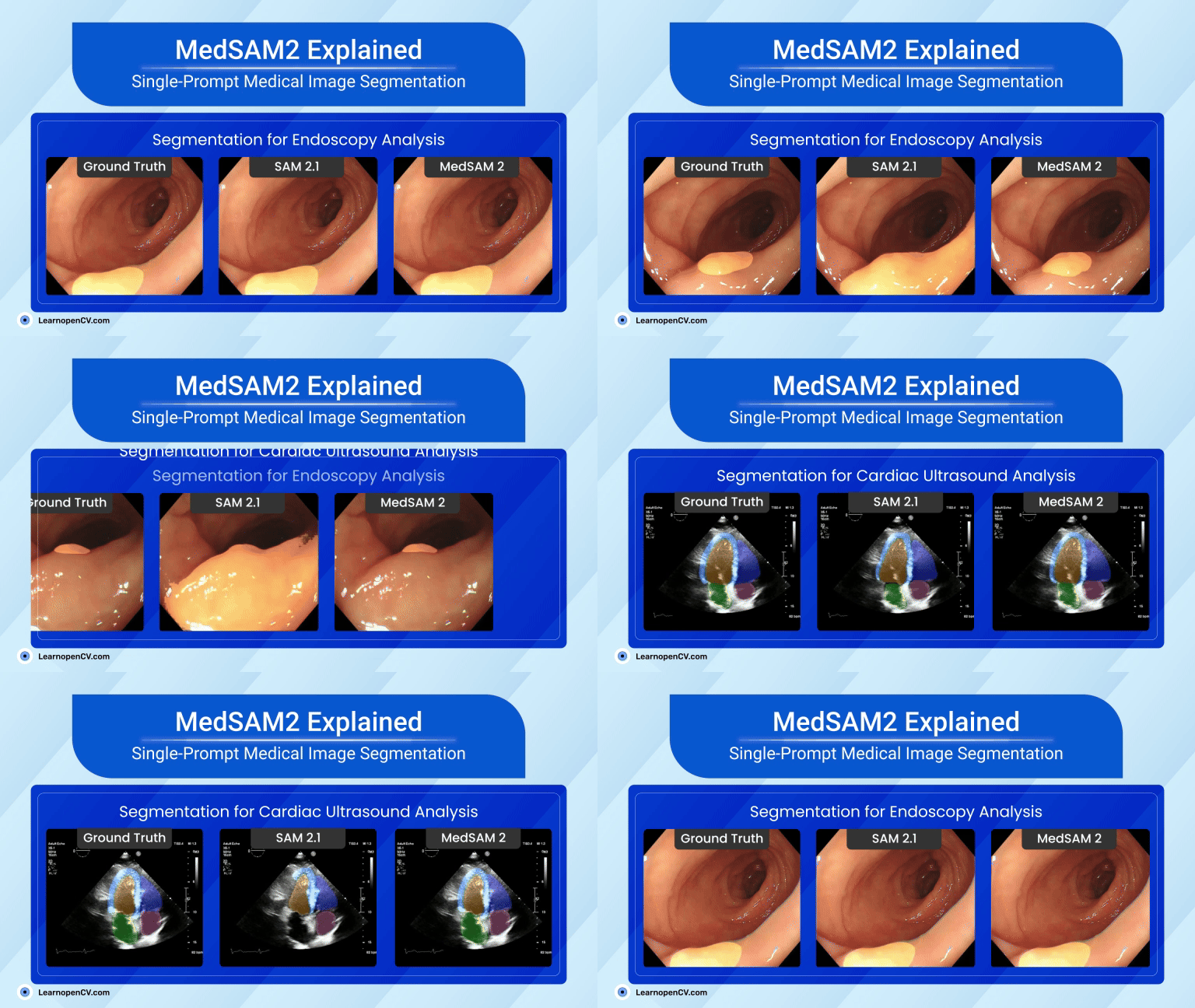
That tiny story shows a significant shift in AI in Healthcare. New MedSAM2, developed by WangLab (the developers of MedSAM), can outline almost any part of any 3D scan or medical video with just one click. Tasks that once took hours now take minutes, providing doctors with faster answers and patients with quicker assistance.
In this article, we will explore:
- Current trends in medical-AI research and why segmentation sits centre-stage.
- What medical imaging really is, and how MedSAM2 will help here.
- A friendly tour of the SAM — MedSAM — SAM2 — MedSAM2 architecture journey.
- Code workflow and inference results.
- A quick recap of the article.
- All the modified Notebooks are given in the Download Code Button.
Now, that’s exciting, right? So grab a cup of coffee, and let’s dive in!
Current Trends in Medical AI
Medical imaging is at the heart of AI’s healthcare boom, and the numbers tell a thriller-style story. In just twelve months, the global AI market in medical imaging jumped from approximately USD 1 billion in 2023 to USD 1.28 billion in 2024; analysts now predict the sector will reach anywhere between USD 14 billion and USD 24 billion by the early 2030s, implying a compound annual growth rate of over 30%.
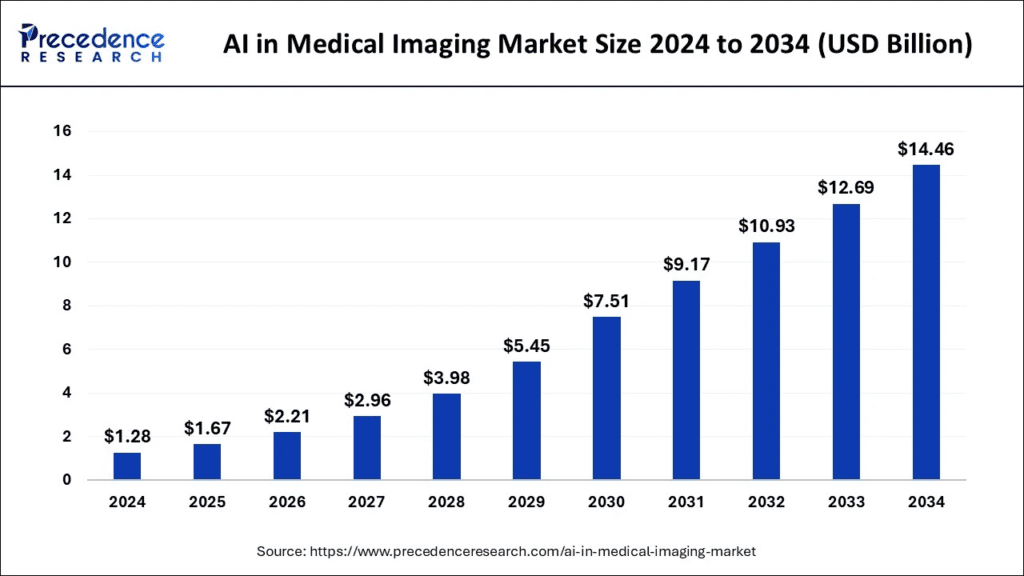
Rise of Foundation models
Why that pace? One word: foundation models. Just as GPT-style language models are rewriting NLP, vision language models (like SAM) are revolutionizing Vision. A recent arXiv survey reveals more than 40 new “segment-anything” spin-offs for medical scans in the past 18 months alone, with conference tracks and entire CVPR workshops emerging to cover them.
Segmentation is the new gateway for Healthcare
Hospitals often adopt AI first for segmentation because it’s concrete, auditable, and meshes with existing workflows. Faster, sharper borders mean:
- Fewer surgical surprises – oncology teams can sculpt radiation beams with sub-millimetre precision.
- Quicker reads in busy ERs – one bounding box on a CT slice, and a model like MedSAM2 outlines the spleen or a bleeding lesion in under a second.
- Better downstream AI – clean masks feed volumetric tumour-growth models or 3-D printing pipelines without manual cleanup.
What is Medical Imaging? How MedSAM2 can help!
Medical imaging is just taking pictures of the inside of the body. X-rays scan bones, CT slices you like a loaf of bread, MRI looks at soft tissue, PET lights up metabolism, and ultrasound films organs in motion. All those pixels let doctors see what the hands can’t feel.
Massive Workload – A single abdominal CT scan can produce over 1,000 slices; an echocardiogram can record the heart beating 60 times a second. Colouring every slice by hand is like painting each frame of an entire Pixar film.
MedSAM2 as a Solution – Drop one click or box, and the model fills in the exact border. From there, doctors can measure tumour volume, steer a radiation beam, or track disease over months.
Four major areas MedSAM2 solves –
| Imaging Task | Old Pain | How MedSAM2 fixes it |
| CT Segmentation | Lesion borders blur into organ tissue. | Hits DSC 0.95 for liver, 0.68 for lesions – about +5 pp over nnU-Net. |
| MRI Segmentation | Variable contrast hides tumours. | Higher median DSC on brain & liver tasks; easily outlines tricky cervical-cancer margins. |
| PET Lesion Detection | Noise and benign uptake cause false positives. | DSC ≈ 0.68, center-of-mass error ~2 mm when fusing PET+CT. |
| Video Segmentation (US & Endoscopy) | Motion blur and speckle kill accuracy. | Polyp DSC 91.3 %; heart-chamber edges stay crisp in real-time echo. |
Now, let’s dive into the Model itself and see how the MedSAM2 was created.
Introduction to MedSAM2
Every major breakthrough often builds upon a strong foundation, and MedSAM2 is no exception. Its development traces back to one of the most influential models in recent computer vision research: Meta AI’s Segment Anything Model 2 (SAM2). SAM demonstrated that a single, prompt-driven network could accurately segment virtually any object within natural images, from animals and vehicles to everyday objects, using minimal user input, such as a single click.
SAM — MedSAM — SAM2 — MedSAM2
SAM (Apr 2023)
Meta AI’s first Segment Anything Model proved that a single click could outline almost any object in a photo. It learned from a billion natural-image masks and turned segmentation into a point-and-paint trick.
MedSAM (Apr 2023)
Researchers at WangLab asked, “What if we fine-tune SAM on hospital scans?” They fine-tuned the model on 1.5 million CT, MRI, and X-ray slices. MedSAM could now color livers and tumors much like SAM colors coffee cups, but only slice by slice, still in pure 2D.
SAM2 (Nov 2024)
Meta’s upgrade retained the click-anywhere spirit but replaced the heavier Hiera transformer backbone with a lighter one, introducing a tidier prompt and mask head that made the network faster and less memory-intensive. SAM2 still thinks in flat frames; it has no built-in way to remember what came before or after a frame in a stack or a clip.
MedSAM2 (Apr 2025)
The newest step combines the best of both worlds. It retains SAM2’s speedy Hiera core and adds a small memory-attention block, allowing every CT slice or video frame to examine its eight neighbors. Trained on a 10-modality mix (≈ 450 k 3-D volumes plus 76 k video frames), MedSAM 2 understands whole volumes and live ultrasound in one go while still running quickly on a regular workstation GPU.
In one sentence: SAM proved the idea, MedSAM made it medical, SAM 2 made it fast, and MedSAM 2 makes it work in full 3-D and real-time video by giving the network a short-term memory.
How MedSAM 2 Works Inside
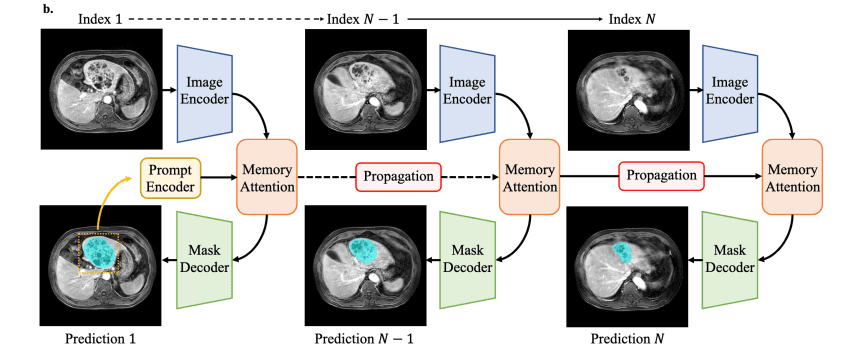
Smaller, faster Input
Images are downsized to 512 × 512 instead of 1024 × 1024, which matches most medical slices and halves the computational load.
Hiera backbone with long-reach Attention
The image encoder is a four-stage Hiera vision transformer. Extra global-attention blocks allow far-apart pixels, such as the two tips of a long vessel, to share information.
Memory for 3D and Video
Above the backbone sit four transformer layers that read from a small memory bank holding the previous slices or frames. Rotary position embeddings inform the model precisely where each feature is located in space or time, ensuring that neighboring slices align cleanly and moving borders do not jitter.
Tiny Prompt Encoder
A tiny prompt encoder changes a user’s box, point, or scribble into vector embeddings the network can follow, like dropping a pin on a map.
Mask Decoder
The mask decoder combines the prompt clues with multi-scale features, generates a 128 × 128 mask, and then scales it back to full size. One set of weights now outlines livers in CT stacks and beating ventricles in echo videos, guided by nothing more than a quick click.
Our courses cover Image Segmentation, Fundamentals of Computer Vision, and Deep Learning in depth. To get started, just click below on any of our free Bootcamps!
Dataset Preparation and Training
Dataset Preparation for MedSAM2
To teach MedSAM 2, the team first built one very large set of scans. It contains approximately 450,000 full 3D studies from reputable sources, including LiTS, BraTS, KiTS, FLARE, TotalSegmentator, AutoPET, and several hospital archives. These cover CT, MRI, and PET, so the model is exposed to a wide range of tissue types, imaging machines, and patient populations. They also added approximately 76,000 video frames from echo and endoscopy sets, such as EchoNet-Dynamic and Hyper-Kvasir, giving the network a sense of moving anatomy.
| Modality | Key public sets used | What they add to the mix |
| CT 3-D | LiTS (liver + tumours), KiTS19 (kidneys), FLARE22 (multi-organ), TotalSegmentator (104 structures) | High-contrast organs and diverse lesions |
| MRI 3-D | BraTS (brain tumours), ACDC (cardiac), CHAOS (abdominal organs), MSD #01–10 | Soft-tissue edges, variable contrast |
| PET/CT | AutoPET, Head-Neck Cancer Seg, MICCAI TOTALSEG-PET subset | Hot vs. cold lesion boundaries |
| Ultrasound video | EchoNet-Dynamic & CAMUS (heart), CLUST (fetal), | Motion + speckle noise |
| Endoscopy video | Hyper-Kvasir, Kvasir-SEG, PolypGen | Polyp shapes, lighting shifts |
Every file went through the same cleaning steps:
- CT slices were resized to one-millimetre cubes and their grey values clipped to normal limits.
- MRI and ultrasound images were scaled so that dark and bright parts sit in a similar range.
- Video clips were cropped to 512×512 pixels and fixed at 30 frames per second.
Older models drew a quick “starter” mask (nnU-Net for 3-D scans, a small Mask R-CNN for video). Human reviewers then opened a web tool that highlighted the shaky parts of each mask in red; they only had to tidy those spots.
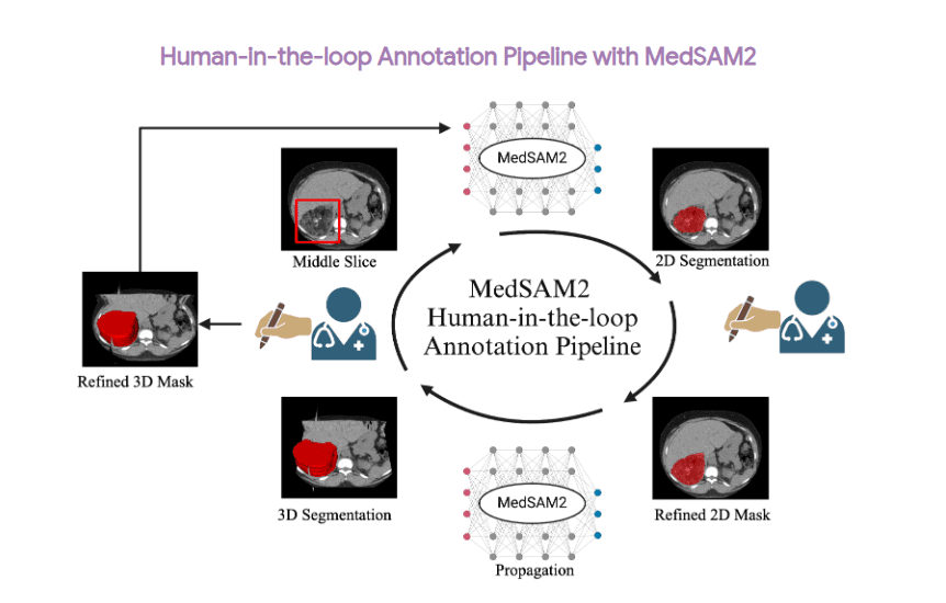
You may have read about three extra datasets in the MedSAM 2 paper: one for CT lesions (DeepLesion), one for MRI liver tumours (LLD-MMRI), and one for echo videos (RVENet). These did not join the big training pool. The authors saved them for later experiments. First, they timed how long doctors needed to correct MedSAM 2’s first-try masks on those scans and showed an 85-92% reduction in labor compared with drawing by hand. Next, they performed a brief additional fine-tuning on the corrected masks, achieving an additional 3-6 Dice points. They also released a MedSAM2-annotated version of these datasets.
MedSAM2 – Training Tweaks
One large mixed dataset – MedSAM 2 trained on approximately 450,000 labelled CT, MRI, and PET scans, as well as 76,000 labelled frames from ultrasound and endoscopy videos. Every file was resized to 512 × 512 (or 1 mm³ voxels for 3D) and placed on the same grayscale scale, so the model never had to guess what “bright” or “dark” meant.
Fast “draft-and-fix” labels – Old networks (nnU-Net for 3D, a small Mask R-CNN for video) drew rough masks. Human reviewers only fixed the messy edges that the software coloured in red. This sped up labelling by a factor of ten.
Balanced batches – CT is common, PET is rare. During training, the loader quietly showed PET and endoscopy slices nearly twice as often and limited any single CT study to 5 % of a batch. That kept the model from turning into a “CT-only” expert.
Now, let’s move on to the code!
Code Pipeline
Now we start playing with the model. For that, we need to clone the official MedSAM2 repository.
git clone https://github.com/bowang-lab/MedSAM2.git && cd MedSAM2
We will then create a virtual environment to run all our experiments.
conda create -n medsam2 python=3.12 -y && conda activate medsam2
Then run this command to install all the requirements
pip install torch torchvision
pip install -e ".[dev]"
One final Step, download the MedSAM2 checkpoints by running:
sh download.sh
We are now finished with the setup; let’s proceed to the main code. We will explore two main applications here.
CT Lesion Segmentation
A CT scan (Computed Tomography scan) is a medical imaging technique that allows doctors to see inside the body with great detail. Unlike regular X-rays that show only a flat image, a CT scan takes many cross-sectional images (called slices) using rotating X-ray beams and a computer to create detailed pictures of bones, organs, blood vessels, and soft tissues. These images can then be viewed individually or reconstructed into a 3D model, giving doctors a clearer understanding of a patient’s condition.
Here we will take 3D CT scan images of the pelvis, viewed in axial slices (horizontal cross-sections). And try to segment a lesion (probably a prostate tumor) with MedSAM2.
Section 1: Imports, Setup, and Argument Parsing
This initial part of the script sets up the necessary environment and obtains user input. It imports various Python libraries required for tasks like file handling (os, glob), numerical operations (numpy), data manipulation (pandas), image processing (PIL, SimpleITK, skimage), deep learning (torch), and plotting (matplotlib).
It also sets random seeds for PyTorch and NumPy to ensure that if you run the script multiple times with the same inputs, you get the same results (reproducibility). The torch.set_..._precision(...) line potentially optimizes matrix multiplication performance on specific newer GPUs.
from glob import glob
from tqdm import tqdm
import os
from os.path import join, basename
import re
import matplotlib.pyplot as plt
from collections import OrderedDict
import pandas as pd
import numpy as np
import argparse

from PIL import Image
import SimpleITK as sitk
import torch
import torch.multiprocessing as mp
from sam2.build_sam import build_sam2_video_predictor_npz # Specific predictor for NPZ input
import SimpleITK as sitk
from skimage import measure, morphology

# Set seeds for reproducibility and configure PyTorch performance
torch.set_float32_matmul_precision('high')
torch.manual_seed(2024)
torch.cuda.manual_seed(2024)
np.random.seed(2024)

# Initialize argument parser
parser = argparse.ArgumentParser()
Next, the script defines command-line arguments using argparse. This allows users to specify different settings when running the script without modifying the code itself.
parser.add_argument(
    '--checkpoint',
    type=str,
    default="checkpoints/MedSAM2_latest.pt",
    help='checkpoint path',
)
parser.add_argument(
    '--cfg',
    type=str,
    default="configs/sam2.1_hiera_t512.yaml",
    help='model config',
)

# more arguments here (skipped)

# Parse the arguments provided from the command line
args = parser.parse_args()
checkpoint = args.checkpoint
model_cfg = args.cfg
imgs_path = args.imgs_path
gts_path = args.gts_path
pred_save_dir = args.pred_save_dir
# Ensure the output directory exists, create if not
os.makedirs(pred_save_dir, exist_ok=True)
propagate_with_box = args.propagate_with_box
This section essentially prepares the script by importing necessary tools, setting up for consistent results, and defining how users can interact with it via the command line to control its behavior and input/output locations. The parsed arguments are then stored in variables for later use.
Section 2: Helper Functions
This section defines several utility functions that are used later in the script for tasks like image preprocessing, creating prompts, post-processing segmentations, and potentially visualization or evaluation.
def getLargestCC(segmentation):
    # Finds connected components in the binary segmentation mask
    labels = measure.label(segmentation)
    # Check if there are any foreground labels (labels > 0)
    if labels.max() == 0: # Handle empty segmentation
        return segmentation # Return the empty segmentation as is
    # Count occurrences of each label (excluding background label 0)
    # Find the label with the largest count (largest connected component)
    largestCC = labels == np.argmax(np.bincount(labels.flat)[1:])+1
    # Return a mask containing only the largest connected component
    return largestCC
getLargestCC(...): This function takes a binary segmentation mask (an array where pixels belonging to the segmented object are 1 and background is 0) and performs post-processing. It identifies all separate “blobs” or connected regions of foreground pixels. It then finds the largest blob (the one with the most pixels) and returns a new mask containing only this largest region.
def dice_multi_class(preds, targets):
    smooth = 1.0
    assert preds.shape == targets.shape
    # Find unique foreground labels in the target mask
    labels = np.unique(targets)[1:]
    dices = []
    for label in labels:
        # Create binary masks for the current label
        pred = preds == label
        target = targets == label
        # Calculate intersection and sum for Dice score
        intersection = (pred * target).sum()
        dices.append((2.0 * intersection + smooth) / (pred.sum() + target.sum() + smooth))
    # Return the average Dice score across all foreground labels
    return np.mean(dices)
dice_multi_class(...): Calculates the Dice Similarity Coefficient (DSC), a common metric for evaluating segmentation performance. It compares the predicted segmentation (preds) with the ground truth (targets). It calculates the DSC for each distinct object label (ignoring background label 0) and returns the average score.
def show_mask(mask, ax, mask_color=None, alpha=0.5):
    # ... (implementation for displaying a mask overlay on an image plot) ...
    if mask_color is not None:
        color = np.concatenate([mask_color, np.array([alpha])], axis=0)
    else:
        color = np.array([251/255, 252/255, 30/255, alpha]) # Default yellow
    h, w = mask.shape[-2:]
    mask_image = mask.reshape(h, w, 1) * color.reshape(1, 1, -1)
    ax.imshow(mask_image)

def show_box(box, ax, edgecolor='blue'):
    # ... (implementation for drawing a bounding box on an image plot) ...
    x0, y0 = box[0], box[1]
    w, h = box[2] - box[0], box[3] - box[1]
    ax.add_patch(plt.Rectangle((x0, y0), w, h, edgecolor=edgecolor, facecolor=(0,0,0,0), lw=2))
show_mask(...) and show_box(...): These are visualization helpers designed to work with matplotlib. show_mask overlays a semi-transparent colored mask onto an image plot (ax), and show_box draws a rectangle (bounding box) onto the plot.
def resize_grayscale_to_rgb_and_resize(array, image_size):
    """
    Resize a 3D grayscale NumPy array to an RGB image and then resize it.

    Parameters:
        array (np.ndarray): Input array of shape (d, h, w). Grayscale slices.
        image_size (int): Desired square size (image_size x image_size).

    Returns:
        np.ndarray: Resized array of shape (d, 3, image_size, image_size). RGB slices.
    """
    d, h, w = array.shape # Depth, Height, Width of the input 3D volume
    # Initialize an empty array for the output
    resized_array = np.zeros((d, 3, image_size, image_size))

    for i in range(d): # Iterate through each slice along the depth dimension
        # Convert the 2D grayscale slice (h, w) to a PIL Image object
        img_pil = Image.fromarray(array[i].astype(np.uint8))
        # Convert the PIL Image to RGB format (duplicates the single channel 3 times)
        img_rgb = img_pil.convert("RGB")
        # Resize the RGB image to the target square size (image_size, image_size)
        img_resized = img_rgb.resize((image_size, image_size))
        # Convert the resized PIL image back to a NumPy array and change layout
        # from (image_size, image_size, 3) to (3, image_size, image_size) for PyTorch
        img_array = np.array(img_resized).transpose(2, 0, 1)
        # Store the processed slice in the output array
        resized_array[i] = img_array

    return resized_array
resize_grayscale_to_rgb_and_resize(...): This is a crucial preprocessing function. SAM2 (like the original SAM) expects RGB images of a specific square size (here, 512×512 based on the config name --cfg configs/sam2.1_hiera_t512.yaml). Medical images, such as CT scans, are often grayscale and have different dimensions. This function takes a 3D NumPy array (Depth, Height, Width) representing the grayscale volume, iterates through each 2D slice, converts it to a 3-channel RGB image (by simply duplicating the grayscale channel), resizes it to the required square image_size, and rearranges the dimensions to the (Channel, Height, Width) format expected by PyTorch models. The output is a 4D NumPy array (depth, 3, image_size, image_size).
def mask2D_to_bbox(gt2D, max_shift=20):
    # ... (implementation for finding the tight bbox around a 2D mask) ...
    # ... (adds optional random coordinate shift) ...
    y_indices, x_indices = np.where(gt2D > 0)
    if len(x_indices) == 0: # Handle empty mask
        return np.array([0, 0, 0, 0]) # Return zero box
    x_min, x_max = np.min(x_indices), np.max(x_indices)
    y_min, y_max = np.min(y_indices), np.max(y_indices)
    H, W = gt2D.shape
    bbox_shift = np.random.randint(0, max_shift + 1, 1)[0]
    x_min = max(0, x_min - bbox_shift)
    x_max = min(W-1, x_max + bbox_shift)
    y_min = max(0, y_min - bbox_shift)
    y_max = min(H-1, y_max + bbox_shift)
    boxes = np.array([x_min, y_min, x_max, y_max]) # XYXY format
    return boxes

def mask3D_to_bbox(gt3D, max_shift=20):
    # ... (implementation for finding the tight bbox around a 3D mask) ...
    # ... (adds optional random coordinate shift) ...
    z_indices, y_indices, x_indices = np.where(gt3D > 0)
    if len(x_indices) == 0: # Handle empty mask
        return np.array([0, 0, 0, 0, 0, 0]) # Return zero box
    x_min, x_max = np.min(x_indices), np.max(x_indices)
    y_min, y_max = np.min(y_indices), np.max(y_indices)
    z_min, z_max = np.min(z_indices), np.max(z_indices)
    D, H, W = gt3D.shape
    bbox_shift = np.random.randint(0, max_shift + 1, 1)[0]
    x_min = max(0, x_min - bbox_shift)
    x_max = min(W-1, x_max + bbox_shift)
    y_min = max(0, y_min - bbox_shift)
    y_max = min(H-1, y_max + bbox_shift)
    z_min = max(0, z_min) # Usually no shift in Z for key slice prompting
    z_max = min(D-1, z_max)
    boxes3d = np.array([x_min, y_min, z_min, x_max, y_max, z_max]) # XYZXYZ format
    return boxes3d
mask2D_to_bbox(...) / mask3D_to_bbox(...): These functions take a 2D or 3D binary mask and calculate the tightest bounding box around the foreground pixels (the object). They find the minimum and maximum x, y (and z for 3D) coordinates containing the object. Optionally, they can add a random “shift” to the box coordinates, slightly expanding the box. This might be used to generate bounding box prompts from existing masks, for example, for training data augmentation or simulating slightly imprecise user input. However, since this script uses propagate_with_box=True by default and gets the box from the CSV file, these mask-to-box functions are likely not used in the standard execution path.
Section 3: Main Processing Loop
This is the core part of the script where the actual segmentation happens. It iterates through each 3D CT scan file found in the input directory.
First, the script loads information about the lesions from the CSV. This file serves as a guide, indicating the locations of lesions within the CT scans, including details such as bounding boxes on specific slices and the optimal contrast settings (DICOM windows) for viewing them. Then, it finds all the 3D CT scan files (.nii.gz) in the folder provided by the user (imgs_path). It cleans up this list to ignore temporary files and prints the number of scans it found.
# Load metadata about lesions from a CSV file.
DL_info = pd.read_csv('CT_DeepLesion/DeepLesion_Dataset_Info.csv')

# Find all '.nii.gz' files in the specified image directory
nii_fnames = sorted(os.listdir(imgs_path))
nii_fnames = [i for i in nii_fnames if i.endswith('.nii.gz')]
# Filter out hidden or temporary files
nii_fnames = [i for i in nii_fnames if not i.startswith('._')]
print(f'Processing {len(nii_fnames)} nii files')

# Initialize an ordered dictionary to store results information
seg_info = OrderedDict()
seg_info['nii_name'] = []
seg_info['key_slice_index'] = []
seg_info['DICOM_windows'] = []

# Initialize the MedSAM2 predictor model
predictor = build_sam2_video_predictor_npz(model_cfg, checkpoint)
Finally, it sets up a dictionary (seg_info) to keep track of the results it generates and initializes the MedSAM2 model using the build_sam2_video_predictor_npz function, loading the specified configuration and pre-trained weights. This predictor is designed to work with sequences of image data, like the slices of a 3D scan.
Section 3.1: Processing Each CT Scan File
The script now enters its main loop, going through each .nii.gz file one by one. For each scan file, it first extracts information from the filename (like the range of slices it covers and a unique case identifier) to help find the corresponding lesion details in the previously loaded DL_info table.
It then loads the actual 3D image data from the .nii.gz file into a NumPy array using the SimpleITK library. It filters the DL_info table to get only the rows that match the current CT scan file. Since one scan might contain multiple lesions listed separately in the CSV, it prepares an empty 3D array (segs_3D_volume) of the same size as the input scan to store the combined segmentation results for all lesions found within this scan.
# Loop through each detected NIfTI file with a progress bar
for nii_fname in tqdm(nii_fnames):
    # --- Start processing one NIfTI file ---

    # Extract slice range and case name from the filename
    range_suffix = re.findall(r'\d{3}-\d{3}', nii_fname)[0]
    slice_range = range_suffix.split('-')
    slice_range = [str(int(s)) for s in slice_range]
    slice_range_str = ', '.join(slice_range) # Format for matching CSV

    # Load the 3D image volume and convert to NumPy array
    nii_image = sitk.ReadImage(join(imgs_path, nii_fname))
    nii_image_data = sitk.GetArrayFromImage(nii_image) # Shape: (Depth, Height, Width)

    case_name = re.findall(r'^(\d{6}_\d{2}_\d{2})', nii_fname)[0]

    # Find matching lesion entries in the CSV for this scan file
    case_df = DL_info[
        DL_info['File_name'].str.contains(case_name) &
        DL_info['Slice_range'].str.contains(slice_range_str)
    ].copy()

    # Initialize an empty 3D array for the combined segmentation mask of this volume
    segs_3D_volume = np.zeros(nii_image_data.shape, dtype=np.uint8)

    # Loop through each lesion found in the CSV for this NIfTI file
    for row_id, row in case_df.iterrows():
        # --- Start processing one lesion within the NIfTI file ---
        # [Lesion processing code follows inside this inner loop]
        # ...
This part organizes the processing by handling one complete 3D scan at a time and preparing to process each lesion listed for that scan individually.
Section 3.2: Preprocessing for a Single Lesion
Inside the inner loop (processing one specific lesion from the CSV), the script performs preprocessing tailored to that lesion. It reads the DICOM window settings (contrast/brightness levels) from the CSV row and applies them to the entire loaded 3D volume (nii_image_data). This clipping and normalization step (np.clip, scaling to 0-255) makes the lesion easier to see according to the metadata.
It then identifies the ‘key slice’ index provided in the CSV and calculates its corresponding index (key_slice_idx_offset) within the loaded NumPy array segment. The bounding box coordinates are also extracted from the CSV and converted into the [x_min, y_min, x_max, y_max] (XYXY) format. The original 3D image data (after windowing/normalization) is stored in img_3D_ori for potential later use (like saving alongside the mask).
# 1. Load Lesion Metadata & Preprocess Image Slice for the Lesion
        lower_bound, upper_bound = row['DICOM_windows'].split(',')
        lower_bound, upper_bound = float(lower_bound), float(upper_bound)

        # Apply windowing and normalize to 0-255 (uint8)
        nii_image_data_pre = np.clip(nii_image_data, lower_bound, upper_bound)
        nii_image_data_pre = (nii_image_data_pre - np.min(nii_image_data_pre))/(np.max(nii_image_data_pre)-np.min(nii_image_data_pre))*255.0
        nii_image_data_pre = np.uint8(nii_image_data_pre)

        # Get key slice index and bounding box
        key_slice_idx_csv = int(row['Key_slice_index'])
        slice_idx_start, slice_idx_end = map(int, row['Slice_range'].split(','))
        key_slice_idx_offset = key_slice_idx_csv - slice_idx_start
        bbox_coords = list(map(int, map(float, row['Bounding_boxes'].split(',')))) # ymin, xmin, ymax, xmax
        bbox_xyxy = np.array([bbox_coords[1], bbox_coords[0], bbox_coords[3], bbox_coords[2]]) # xmin, ymin, xmax, ymax

        # Store the preprocessed 3D volume data for this lesion
        img_3D_ori = nii_image_data_pre
        assert np.max(img_3D_ori) < 256, f'Input data should be uint8 range [0, 255]'

        # Get original height/width for resizing outputs later
        key_slice_img = nii_image_data_pre[key_slice_idx_offset, :,:]
        video_height, video_width = key_slice_img.shape[0], key_slice_img.shape[1]
This step focuses on preparing the image data based on the specific lesion’s metadata, ensuring optimal contrast, and extracting the necessary prompt information (the bounding box).
Section 3.3: Preparing Input Tensor for MedSAM2
After basic preprocessing, the data needs further transformation to match the MedSAM2 model’s expected input format. The resize_grayscale_to_rgb_and_resize function is called to convert the 3D grayscale volume (img_3D_ori) into a stack of 512×512 RGB images (even though the original was grayscale, the model expects 3 channels).
The pixel values are scaled to the range [0.0, 1.0]. This NumPy array is then converted into a PyTorch tensor and moved to the GPU (cuda). Finally, standard ImageNet normalization (subtracting the mean and dividing by the standard deviation for each channel) is applied. The result (img_resized) is a tensor ready to be fed into the MedSAM2 predictor.
# 2. Prepare Input for MedSAM2 Model
        # Resize slices to 512x512 and convert to RGB format
        img_resized = resize_grayscale_to_rgb_and_resize(img_3D_ori, 512) # Shape: (D, 3, 512, 512)
        # Normalize pixel values to 0.0-1.0
        img_resized = img_resized / 255.0
        # Convert to PyTorch tensor and move to GPU
        img_resized = torch.from_numpy(img_resized).cuda()

        # Define and apply ImageNet normalization
        img_mean=(0.485, 0.456, 0.406)
        img_std=(0.229, 0.224, 0.225)
        img_mean = torch.tensor(img_mean, dtype=torch.float32)[:, None, None].cuda()
        img_std = torch.tensor(img_std, dtype=torch.float32)[:, None, None].cuda()
        img_resized -= img_mean
        img_resized /= img_std
This is the final preparation step before the actual segmentation, ensuring the data dimensions, format, and value ranges are exactly what the deep learning model expects.
Section 4: Running MedSAM2 Inference
Now, the core segmentation process begins for the current lesion. An empty 3D NumPy array (segs_3D_lesion) is created to store the segmentation mask specifically for this lesion. The code uses torch.inference_mode() and torch.autocast for optimized performance during inference (faster computation, potentially lower memory use with bfloat16).
First, the predictor.init_state method is called with the preprocessed image tensor (img_resized). This likely calculates and stores the initial image embeddings for the volume. Then, the bounding box (bbox_xyxy) identified earlier is provided as a prompt on the key slice (key_slice_idx_offset) using predictor.add_new_points_or_box.
The script then calls predictor.propagate_in_video to perform segmentation propagation forward from the key slice towards the end of the volume. This function iterates through the slices, using the model’s internal memory to maintain consistency. For each slice (out_frame_idx), it returns the mask logits (out_mask_logits). These logits are thresholded (at 0.0) to create a binary mask, which is then used to mark the corresponding pixels in the segs_3D_lesion array.
After the forward pass, the predictor’s internal state (memory) is reset using predictor.reset_state. The initial bounding box prompt is added again to the key slice. Then, predictor.propagate_in_video(...) is called to propagate segmentation backward from the key slice towards the beginning of the volume. The resulting binary masks are again used to update the segs_3D_lesion array. Using logical OR ensures that pixels segmented in either the forward or backward pass are included in the final lesion mask. Finally, the predictor state is reset one last time.
 # 3. Run MedSAM2 Inference for the current lesion
        segs_3D_lesion = np.zeros(nii_image_data.shape, dtype=np.uint8) # Mask for this specific lesion

        # Use inference mode and mixed precision for efficiency
        with torch.inference_mode(), torch.autocast("cuda", dtype=torch.bfloat16):
            # Initialize predictor state with the volume data
            inference_state = predictor.init_state(img_resized, video_height, video_width)

            # Add the initial bounding box prompt on the key slice
            if propagate_with_box:
                predictor.add_new_points_or_box(
                    inference_state=inference_state,
                    frame_idx=key_slice_idx_offset,
                    obj_id=1, # Assign ID 1 to this lesion object
                    box=bbox_xyxy,
                )
            else: # gt (Alternative prompting not used by default)
                pass

            # Propagate segmentation FORWARD from the key slice
            for out_frame_idx, _, out_mask_logits in predictor.propagate_in_video(inference_state):
                binary_mask = (out_mask_logits[0] > 0.0).cpu().numpy()[0]
                segs_3D_lesion[out_frame_idx, binary_mask] = 1 # Mark segmented pixels

            # Reset predictor state (clear memory) before backward pass
            predictor.reset_state(inference_state)

            # Add the initial prompt AGAIN for the backward pass
            if propagate_with_box:
                 predictor.add_new_points_or_box(
                    inference_state=inference_state,
                    frame_idx=key_slice_idx_offset,
                    obj_id=1,
                    box=bbox_xyxy,
                )
            else: # gt
                pass

            # Propagate segmentation BACKWARD from the key slice
            for out_frame_idx, _, out_mask_logits in predictor.propagate_in_video(inference_state, reverse=True):
                binary_mask = (out_mask_logits[0] > 0.0).cpu().numpy()[0]
                segs_3D_lesion[out_frame_idx, binary_mask] = 1 # Update mask (union)

            # Reset state after finishing this lesion
            predictor.reset_state(inference_state)
This bidirectional propagation is the key step where MedSAM2 uses the initial prompt and its temporal consistency mechanisms to segment the lesion across multiple slices.
Section 4.1: Post-processing and Combining Results
After the forward and backward propagation for a single lesion, the resulting mask (segs_3D_lesion) might contain small, disconnected regions or noise. The script checks if any segmentation actually happened (np.max(segs_3D_lesion) > 0). If so, it calls the getLargestCC function to perform post-processing, keeping only the largest connected component of the segmented pixels.
This cleans up the result. Then, this cleaned-up mask for the current lesion is combined with the main segmentation mask for the entire NIfTI volume (segs_3D_volume) using a logical OR operation. This ensures that if multiple lesions are processed for the same scan file, their segmentations are accumulated into the final output mask.
# 4. Post-process the segmentation for the current lesion
        if np.max(segs_3D_lesion) > 0:
            # Keep only the largest connected component (removes noise)
            segs_3D_lesion = getLargestCC(segs_3D_lesion)
            segs_3D_lesion = np.uint8(segs_3D_lesion)

        # 5. Combine the current lesion's segmentation with the volume's segmentation
        # Use logical OR to merge masks if multiple lesions exist in the volume
        segs_3D_volume = np.logical_or(segs_3D_volume, segs_3D_lesion).astype(np.uint8)

    # --- End processing one lesion --- (Inner loop finishes here) ---
This step refines the individual lesion segmentation and merges it into the final output for the entire scan volume.
Section 4.2: Saving Final Results
Once the inner loop finishes (meaning all lesions listed for the current NIfTI file in the CSV have been processed and their masks combined into segs_3D_volume), the script saves the results. It converts the final NumPy segmentation array (segs_3D_volume) back into a SimpleITK image object. Critically, it copies the spatial metadata (like spacing, origin, and orientation) from the original input NIfTI image (nii_image) to the new mask image (sitk_mask). This ensures the saved mask aligns correctly with the original scan in medical viewers.
It also saves the preprocessed (windowed) version of the input image (img_3D_ori from the last lesion processed) for reference. Filenames are constructed based on the original input filename, adding suffixes like _img.nii.gz and _mask.nii.gz (incorporating the key slice index from the last lesion into the mask filename). Finally, it records information about the saved mask file (filename, key slice index, DICOM window used for the last lesion) into the seg_info dictionary.
# --- End processing one NIfTI file --- (Outer loop continues after this) ---

    # 6. Save Results for the entire NIfTI volume
    # Convert final NumPy mask to SimpleITK image
    sitk_mask = sitk.GetImageFromArray(segs_3D_volume)
    # Copy spatial metadata from original NIfTI
    sitk_mask.CopyInformation(nii_image)

    # Prepare the preprocessed image (from last lesion) for saving
    sitk_image_preprocessed = sitk.GetImageFromArray(img_3D_ori)
    sitk_image_preprocessed.CopyInformation(nii_image)

    # Define output filenames
    key_slice_idx_csv = int(row['Key_slice_index']) # Key slice from the last processed row
    save_seg_name = nii_fname.split('.nii.gz')[0] + f'_k{key_slice_idx_csv}_mask.nii.gz'
    save_img_name = nii_fname.replace('.nii.gz', '_img.nii.gz')

    # Write the preprocessed image and the final segmentation mask to disk
    sitk.WriteImage(sitk_image_preprocessed, os.path.join(pred_save_dir, save_img_name))
    sitk.WriteImage(sitk_mask, os.path.join(pred_save_dir, save_seg_name))

    # Record metadata about the saved segmentation
    seg_info['nii_name'].append(save_seg_name)
    seg_info['key_slice_index'].append(key_slice_idx_csv)
    seg_info['DICOM_windows'].append(row['DICOM_windows'])

# --- (Outer loop continues to the next nii_fname) ---
This is where the final output for each processed CT scan volume, along with relevant metadata, is generated and stored.
Section 4.3: Saving Summary Information
After the main outer loop has finished processing all the NIfTI files in the input directory, the script takes the seg_info dictionary, which has collected the filename, key slice index, and DICOM window for each generated segmentation mask, and converts it into a Pandas DataFrame. This DataFrame is then saved as a CSV file (named tiny_seg_info202412.csv in the specified output directory). This summary file provides a convenient way to track which output mask corresponds to which input file and key slice prompt.
# After processing all NIfTI files, save the collected segmentation info to a CSV
seg_info_df = pd.DataFrame(seg_info)
seg_info_df.to_csv(join(pred_save_dir, 'tiny_seg_info202412.csv'), index=False)
And here is the result:
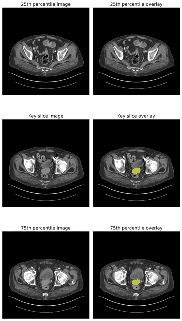
You can see the model has segmented a small structure in the pelvis, most likely the bladder or possibly a prostate tumor or pelvic mass, depending on the clinical task. Isn’t it cool! This can save a lot of time for doctors and surgeons, helping them make decisions quickly, which can save millions of lives and make our healthcare system smarter and more efficient.
Video Segmentation – Heart Echo
In this section, we will use an echocardiogram (or “echo”) video of a patient to examine the heart, like the left ventricle (the main pumping chamber), its muscle wall, and nearby areas.
An echocardiogram(A specialized type of ultrasound that focuses specifically on imaging the heart) image, specifically, it appears to be a 4-chamber (4CH) view of the heart, often used in cardiac ultrasound (echocardiography).
In a 4CH view, you typically visualize:
- The left and right atria (top chambers)
- The left and right ventricles (bottom chambers)
- The interatrial and interventricular septa (walls separating chambers)
We will try with this 4CH video and see how MedSAM2 segments the heart components.
Section 1: Imports and Setup
This part imports the necessary libraries, including argparse, os, collections, defaultdict, NumPy, and PyTorch. It specifically imports build_sam2_video_predictor from the MedSAM2 library, which is the main class responsible for handling video segmentation inference.
# Copyright (c) Meta Platforms, Inc. and affiliates.
# All rights reserved.

# This source code is licensed under the license found in the
# LICENSE file in the root directory of this source tree.

import argparse
import os
from collections import defaultdict

import numpy as np
import torch
from PIL import Image
from sam2.build_sam import build_sam2_video_predictor

# the PNG palette for DAVIS 2017 dataset
DAVIS_PALETTE = b"\x00\x00\\...@`\xe0@\xe0\xe0@``\xc0\xe0`\xc0`\xe0\xc0\xe0\xe0\xc0"
The script also defines DAVIS_PALETTE, which is a specific color map (palette) used in the DAVIS 2017 video segmentation benchmark dataset. This palette allows saving multi-object segmentation masks as a single PNG image where each object ID corresponds to a unique color. This is useful for visualization and evaluation on standard benchmarks.
Section 2: Helper Functions for PNG Mask Handling
This section defines several functions specifically for reading and writing segmentation masks stored as PNG image files. These formats are common in video object segmentation datasets.
def load_ann_png(path):
    """Load a PNG file as a mask and its palette."""
    # Open the PNG image file using PIL
    mask = Image.open(path)
    # Get the color palette embedded in the PNG (if it exists)
    palette = mask.getpalette()
    # Convert the PIL image to a NumPy array of unsigned 8-bit integers (uint8)
    mask = np.array(mask).astype(np.uint8)
    # Return both the mask data (as a NumPy array) and the palette
    return mask, palette
load_ann_png(...): This function reads a PNG file that’s expected to be a segmentation mask, often using a specific color palette (like the DAVIS_PALETTE defined earlier). It uses the Pillow (PIL) library to open the image, extracts the mask data as a NumPy array (where pixel values typically represent object IDs), and also extracts the color palette associated with the image.
def save_ann_png(path, mask, palette):
    """Save a mask as a PNG file with the given palette."""
    # Ensure the mask data is uint8 and 2-dimensional (Height x Width)
    assert mask.dtype == np.uint8
    assert mask.ndim == 2
    # Convert the NumPy array back to a PIL Image object
    output_mask = Image.fromarray(mask)
    # Apply the provided color palette to the image
    output_mask.putpalette(palette)
    # Save the image to the specified path
    output_mask.save(path)
save_ann_png(...): This is the counterpart to load_ann_png. It takes a NumPy array representing a mask and a color palette, creates a PIL Image object from the mask data, applies the palette to it, and saves it as a PNG file at the given path.
def get_per_obj_mask(mask):
    """Split a mask into per-object masks."""
    # Find all unique pixel values (object IDs) in the mask
    object_ids = np.unique(mask)
    # Filter out the background ID (usually 0)
    object_ids = object_ids[object_ids > 0].tolist()
    # Create a dictionary: key is object ID, value is a binary (True/False) mask
    # where True indicates pixels belonging to that specific object ID.
    per_obj_mask = {object_id: (mask == object_id) for object_id in object_ids}
    return per_obj_mask
get_per_obj_mask(...): This function takes a mask (like one loaded by load_ann_png) where different objects are represented by different pixel values (e.g., object 1 is value 1, object 2 is value 2). It identifies all unique non-zero object IDs present and creates a dictionary. Each key in the dictionary is an object ID, and the corresponding value is a binary (True/False) mask indicating only the pixels belonging to that specific object.
def put_per_obj_mask(per_obj_mask, height, width):
    """Combine per-object masks into a single mask."""
    # Create an empty mask filled with zeros (background)
    mask = np.zeros((height, width), dtype=np.uint8)
    # Get object IDs from the input dictionary, sort them in reverse order
    # (so higher IDs overwrite lower IDs if masks overlap, common in VOS)
    object_ids = sorted(per_obj_mask)[::-1]
    for object_id in object_ids:
        # Get the binary mask for the current object ID
        object_mask = per_obj_mask[object_id]
        # Ensure it has the correct shape (Height x Width)
        object_mask = object_mask.reshape(height, width)
        # Assign the object ID value to the pixels where the binary mask is True
        mask[object_mask] = object_id
    return mask
put_per_obj_mask(...): This does the reverse. It takes a dictionary of binary masks (like the one produced by get_per_obj_mask or the output from the model) and combines them into a single mask image. Pixels belonging to object ID n will be assigned the value n in the output mask. It handles potential overlaps by processing objects in reverse sorted order of IDs, meaning higher IDs take precedence.
def load_masks_from_dir(
    input_mask_dir, video_name, frame_name, per_obj_png_file, allow_missing=False
):
    """Load masks from a directory as a dict of per-object masks."""
    # Case 1: Masks are combined in a single palettized PNG per frame (like DAVIS)
    if not per_obj_png_file:
        input_mask_path = os.path.join(input_mask_dir, video_name, f"{frame_name}.png")
        # Optionally skip if the mask file doesn't exist
        if allow_missing and not os.path.exists(input_mask_path):
            return {}, None
        # Load the combined mask and its palette
        input_mask, input_palette = load_ann_png(input_mask_path)
        # Split into individual binary masks per object
        per_obj_input_mask = get_per_obj_mask(input_mask)
    # Case 2: Each object has its own PNG file in a subdirectory (like SA-V)
    else:
        per_obj_input_mask = {}
        input_palette = None # Palette is not usually stored per-object
        # Iterate through object subdirectories (named like '001', '002', ...)
        for object_name in os.listdir(os.path.join(input_mask_dir, video_name)):
            object_id = int(object_name)
            input_mask_path = os.path.join(
                input_mask_dir, video_name, object_name, f"{frame_name}.png"
            )
            # Optionally skip if the mask file doesn't exist
            if allow_missing and not os.path.exists(input_mask_path):
                continue
            # Load the individual object mask (palette might be loaded but usually ignored)
            input_mask, input_palette = load_ann_png(input_mask_path)
            # Store the binary mask (pixels > 0 are foreground)
            per_obj_input_mask[object_id] = input_mask > 0

    return per_obj_input_mask, input_palette
load_masks_from_dir(...): This is a higher-level function that uses the previous helpers. It reads mask information for a specific frame_name within a video_name directory. It adapts its behavior based on the per_obj_png_file flag:
- If False (default), it expects a single PNG file (like
frame_name.png)containing all object masks distinguished by pixel values (like DAVIS format). It usesload_ann_pngandget_per_obj_mask. - If True, it expects subdirectories for each object (e.g., 001/, 002/) inside the video directory, each containing individual PNG mask files (
frame_name.png). It loads these individual files. It returns a dictionary of binary masks per object ID and potentially the palette from the input.
def save_palette_masks_to_dir(
    output_mask_dir,
    video_name,
    frame_name,
    per_obj_output_mask,
    height,
    width,
    per_obj_png_file,
    output_palette,
):
    """Save masks to a directory as PNG files with palette."""
    # Create the output directory for the video if it doesn't exist
    os.makedirs(os.path.join(output_mask_dir, video_name), exist_ok=True)
    # Case 1: Save as a single combined palettized PNG
    if not per_obj_png_file:
        # Combine binary masks into a single mask with object IDs as pixel values
        output_mask = put_per_obj_mask(per_obj_output_mask, height, width)
        output_mask_path = os.path.join(
            output_mask_dir, video_name, f"{frame_name}.png"
        )
        # Save the combined mask using the specified palette
        save_ann_png(output_mask_path, output_mask, output_palette)
    # Case 2: Save each object's mask as a separate PNG
    else:
        for object_id, object_mask in per_obj_output_mask.items():
            object_name = f"{object_id:03d}" # Format object ID (e.g., 1 -> '001')
            # Create subdirectory for the object if needed
            os.makedirs(
                os.path.join(output_mask_dir, video_name, object_name),
                exist_ok=True,
            )
            # Reshape the binary mask and convert to uint8
            output_mask = object_mask.reshape(height, width).astype(np.uint8)
            output_mask_path = os.path.join(
                output_mask_dir, video_name, object_name, f"{frame_name}.png"
            )
            # Save the individual object mask with the palette
            # (Note: palette might not be meaningful here, but function requires it)
            save_ann_png(output_mask_path, output_mask, output_palette)
save_palette_masks_to_dir(...): Saves the predicted masks (per_obj_output_mask, which is a dictionary of binary masks) as PNG files with a color palette (either the one loaded from the input or the default DAVIS_PALETTE). It also handles the two storage formats based on per_obj_png_file: either combining masks into one palettized PNG using put_per_obj_mask, and save_ann_png, or saving each object’s binary mask into its respective subdirectory as a separate palettized PNG.
def save_masks_to_dir(
    output_mask_dir,
    video_name,
    frame_name,
    per_obj_output_mask,
    height,
    width,
    per_obj_png_file,
):
    """Save masks to a directory as greyscale PNG files (no palette)."""
    # Create the output directory for the video if it doesn't exist
    os.makedirs(os.path.join(output_mask_dir, video_name), exist_ok=True)
    # Case 1: Save as a single combined grayscale PNG
    if not per_obj_png_file:
        # Combine binary masks into a single mask with object IDs as pixel values
        output_mask = put_per_obj_mask(per_obj_output_mask, height, width)
        output_mask_path = os.path.join(
            output_mask_dir, video_name, f"{frame_name}.png"
        )
        # Ensure correct data type and dimensions
        assert output_mask.dtype == np.uint8
        assert output_mask.ndim == 2
        # Convert to PIL Image and save (will be grayscale based on object IDs)
        output_mask = Image.fromarray(output_mask)
        output_mask.save(output_mask_path)
    # Case 2: Save each object's mask as a separate grayscale PNG
    else:
        for object_id, object_mask in per_obj_output_mask.items():
            object_name = f"{object_id:03d}" # Format object ID
            # Create subdirectory for the object if needed
            os.makedirs(
                os.path.join(output_mask_dir, video_name, object_name),
                exist_ok=True,
            )
            # Reshape binary mask, convert to uint8 (True becomes 1, False becomes 0)
            output_mask = object_mask.reshape(height, width).astype(np.uint8)
            output_mask_path = os.path.join(
                output_mask_dir, video_name, object_name, f"{frame_name}.png"
            )
            # Ensure correct data type and dimensions
            assert output_mask.dtype == np.uint8
            assert output_mask.ndim == 2
            # Convert to PIL Image and save (will be grayscale, mostly 0s and 1s)
            output_mask = Image.fromarray(output_mask)
            output_mask.save(output_mask_path)
save_masks_to_dir(...): This function is similar to save_palette_masks_to_dir, but it saves the output masks as grayscale PNGs without applying a color palette. In the combined format, the pixel value will be the object ID. In the per-object format, the pixel value will typically be 1 for the object and 0 for the background. This might be used for storing raw predictions before visualization or evaluation that requires a specific palette format.
These functions provide the necessary tools to handle the input mask prompts and save the output segmentations in standard formats commonly used for video object segmentation tasks.
Section 3: VOS Inference
Section 3.1: VOS Inference (Standard Case)
This section defines the vos_inference function, which handles the standard video object segmentation task. It assumes that all objects you want to track are present and visible in the initial frame(s) for which you provide masks. The decorators @torch.inference_mode(...) and @torch.autocast(...) tell PyTorch to optimize for inference (e.g., by not tracking gradients) and to automatically use lower-precision calculations (like bfloat16) if possible, making it run faster and use less memory on compatible GPUs.
@torch.inference_mode()
@torch.autocast(device_type="cuda", dtype=torch.bfloat16)
def vos_inference(
    predictor,            # The initialized MedSAM2 video predictor model
    base_video_dir,       # Directory containing folders of video frames
    input_mask_dir,       # Directory containing folders of input masks (PNGs)
    output_mask_dir,      # Directory where output masks will be saved
    video_name,           # Name of the specific video folder to process
    score_thresh=0.0,     # Threshold for converting logits to binary masks (default 0.0)
    use_all_masks=False,  # If True, use masks from all frames in input_mask_dir as prompts
                          # If False (default), only use the mask from the very first frame
    per_obj_png_file=False, # If True, input/output masks are one PNG per object per frame
                          # If False (default), masks are one combined PNG per frame
    save_palette_png=False, # If True, save output masks with a color palette
                          # If False (default), save as grayscale masks
):
    """Run inference on a single video with the given predictor."""
    # Construct the full path to the video frames directory
    video_dir = os.path.join(base_video_dir, video_name)
    # Get a sorted list of frame filenames (without extension)
    frame_names = [
        os.path.splitext(p)[0]
        for p in os.listdir(video_dir)
        if os.path.splitext(p)[-1] in [".jpg", ".jpeg", ".JPG", ".JPEG"]
    ]
    frame_names = list(sorted(frame_names))

    # Initialize the predictor's internal state for this video. This involves
    # loading the video frames (potentially asynchronously) and preparing the model.
    inference_state = predictor.init_state(
        video_path=video_dir, async_loading_frames=False # False means load all frames now
    )
    # Store the video dimensions for later use when saving masks
    height = inference_state["video_height"]
    width = inference_state["video_width"]
    input_palette = None # Will store the palette if loaded from input mask
This initial part sets up the function, finds all the frame image files for the specified video, and initializes the MedSAM2 predictor’s state, which includes loading the video frames and getting their dimensions.
Next, the function determines which frame(s) contain the initial mask prompts that will guide the segmentation. By default (use_all_masks=False), it assumes only the very first frame (frame_names[0]) has an input mask. If use_all_masks=True, it searches the input_mask_dir for all available mask files for this video, and uses all of them as initial prompts. The indices of these prompt frames are stored in input_frame_inds.
# fetch mask inputs from input_mask_dir (either only mask for the first frame, or all available masks)
    if not use_all_masks:
        # Default: use only the first frame's mask as the input prompt
        input_frame_inds = [0]
    else:
        # Option: use all available mask files as input prompts
        if not per_obj_png_file: # Case 1: Combined mask PNG per frame
            input_frame_inds = [
                idx
                for idx, name in enumerate(frame_names)
                # Check if a mask file exists for this frame index
                if os.path.exists(
                    os.path.join(input_mask_dir, video_name, f"{name}.png")
                )
            ]
        else: # Case 2: Separate mask PNG per object per frame
            input_frame_inds = [
                idx
                # Iterate through object subdirectories
                for object_name in os.listdir(os.path.join(input_mask_dir, video_name))
                # Iterate through frame indices and names
                for idx, name in enumerate(frame_names)
                # Check if a mask file exists for this object and frame index
                if os.path.exists(
                    os.path.join(input_mask_dir, video_name, object_name, f"{name}.png")
                )
            ]
        # Ensure at least one input mask was found
        if len(input_frame_inds) == 0:
            raise RuntimeError(
                f"In {video_name=}, got no input masks in {input_mask_dir=}. "
                "Please make sure the input masks are available in the correct format."
            )
        # Get unique frame indices and sort them
        input_frame_inds = sorted(set(input_frame_inds))
This logic allows flexibility in how the initial segmentation guidance is provided – either just the first frame or multiple frames spread throughout the video.
Now, the script iterates through the identified input_frame_inds. For each prompt frame, it uses the load_masks_from_dir helper function (explained in the previous section) to load the mask(s). It gets back a dictionary per_obj_input_mask where keys are object IDs and values are binary masks. It also checks if any new object IDs appear in later prompt frames that weren’t in the very first one – this standard vos_inference function assumes all objects are present initially and raises an error if this isn’t true (suggesting the user should use the other inference function or a flag). For each object mask loaded, it calls predictor.add_new_mask to feed this initial guidance into the MedSAM2 model’s state for that specific object ID and frame index.
 # add those input masks to SAM 2 inference state before propagation
    object_ids_set = None # To keep track of all object IDs seen so far
    for input_frame_idx in input_frame_inds:
        try:
            # Load mask(s) for the current prompt frame
            per_obj_input_mask, input_palette = load_masks_from_dir(
                input_mask_dir=input_mask_dir,
                video_name=video_name,
                frame_name=frame_names[input_frame_idx],
                per_obj_png_file=per_obj_png_file,
            )
        except FileNotFoundError as e:
            # Handle error if a mask file is expected but not found
            raise RuntimeError(
                f"In {video_name=}, failed to load input mask for frame {input_frame_idx=}. "
                "Please add the `--track_object_appearing_later_in_video` flag "
                # ... (rest of error message) ...
            ) from e

        # Get the set of object IDs from the first prompt frame encountered
        if object_ids_set is None:
            object_ids_set = set(per_obj_input_mask)

        # Add each loaded object mask to the predictor's state
        for object_id, object_mask in per_obj_input_mask.items():
            # Check if a new object ID appears only in a later frame (not allowed here)
            if object_id not in object_ids_set:
                raise RuntimeError(
                    f"In {video_name=}, got a new {object_id=} appearing only in a "
                    f"later {input_frame_idx=} (but not appearing in the first frame). "
                    # ... (rest of error message) ...
                )
            # Add the mask to the predictor state
            predictor.add_new_mask(
                inference_state=inference_state,
                frame_idx=input_frame_idx,
                obj_id=object_id,
                mask=object_mask, # This is the binary mask (True/False)
            )

    # Check if any objects were actually loaded
    if object_ids_set is None or len(object_ids_set) == 0:
        raise RuntimeError(
            f"In {video_name=}, got no object ids on {input_frame_inds=}. "
            # ... (rest of error message) ...
        )
After loading all initial prompts, the script is ready to track the objects through the rest of the video.
The core tracking happens in the predictor.propagate_in_video loop. This function internally iterates through all frames of the video (starting from the earliest prompt frame). For each frame (out_frame_idx), it uses the MedSAM2 model (with its memory mechanism) to predict the masks for all the objects it’s currently tracking (out_obj_ids). It returns the raw prediction scores (logits) for each object (out_mask_logits). The script then converts these logits into binary masks by comparing them against the score_thresh (defaulting to 0.0). These binary masks are stored in the video_segments dictionary, keyed by the frame index.
# run propagation throughout the video and collect the results in a dict
    os.makedirs(os.path.join(output_mask_dir, video_name), exist_ok=True)
    # Use the palette from input if available, otherwise default to DAVIS palette
    output_palette = input_palette or DAVIS_PALETTE
    video_segments = {}  # Stores per-frame segmentation results {frame_idx: {obj_id: mask}}

    # The main loop where the model propagates masks frame by frame
    for out_frame_idx, out_obj_ids, out_mask_logits in predictor.propagate_in_video(
        inference_state
    ):
        # Convert predicted logits to binary masks for each object
        per_obj_output_mask = {
            out_obj_id: (out_mask_logits[i] > score_thresh).cpu().numpy()
            for i, out_obj_id in enumerate(out_obj_ids)
        }
        # Store the binary masks for the current frame
        video_segments[out_frame_idx] = per_obj_output_mask
This loop performs the actual segmentation across the video sequence using the model’s temporal consistency features.
Finally, the script iterates through the collected video_segments. For each frame, it takes the dictionary of per-object binary masks and saves them to the output_mask_dir. Depending on the save_palette_png flag, it either calls save_palette_masks_to_dir (to save potentially colorful, combined, or separate PNGs using a palette) or save_masks_to_dir (to save grayscale PNGs without a palette). The per_obj_png_file flag again determines whether the output is a single combined mask file per frame or separate files per object per frame.
# write the output masks as palette PNG files to output_mask_dir
    for out_frame_idx, per_obj_output_mask in video_segments.items():
        if save_palette_png:
            # Option 1: save palette PNG prediction results
            save_palette_masks_to_dir(
                output_mask_dir=output_mask_dir,
                video_name=video_name,
                frame_name=frame_names[out_frame_idx], # Use original frame name
                per_obj_output_mask=per_obj_output_mask, # Dict of {obj_id: binary_mask}
                height=height,
                width=width,
                per_obj_png_file=per_obj_png_file, # Save format flag
                output_palette=output_palette,    # Palette to use
            )
        else:
            # Option 2: save raw grayscale prediction results (no palette)
            save_masks_to_dir(
                output_mask_dir=output_mask_dir,
                video_name=video_name,
                frame_name=frame_names[out_frame_idx],
                per_obj_output_mask=per_obj_output_mask,
                height=height,
                width=width,
                per_obj_png_file=per_obj_png_file,
            )
This function provides the standard workflow for VOS, where the initial frame contains all necessary object information.
Section 3.2: VOS Inference (Objects Appearing Later)
This section defines vos_separate_inference_per_object, designed for VOS datasets where new objects might appear later in the video (not just in the first frame), like LVOS or YouTube-VOS. The key difference is that it runs the tracking process independently for each object, starting from the frame where that object first appears.
    # --- Collects all masks for all objects across all frames first ---
    inputs_per_object = defaultdict(dict)
    for idx, name in enumerate(frame_names):
        # ... (loads masks for frame 'idx') ...
        for object_id, object_mask in per_obj_input_mask.items():
            # ... (stores mask in inputs_per_object[object_id][idx]) ...

    # --- Runs inference separately for each object ---
    object_ids = sorted(inputs_per_object)
    output_scores_per_object = defaultdict(dict) # Store raw scores per object
    for object_id in object_ids:
        input_frame_inds = sorted(inputs_per_object[object_id]) # Frames for this object
        predictor.reset_state(inference_state) # <<< Reset state for each object
        for input_frame_idx in input_frame_inds:
            # Add only this object's mask(s)
            predictor.add_new_mask(
                # ...
            )

        # Propagate starting from this object's first appearance
        for out_frame_idx, _, out_mask_logits in predictor.propagate_in_video(
            inference_state,
            start_frame_idx=min(input_frame_inds), # <<< Start from object's first frame
            # ...
        ):
            # Store raw scores (logits) for this object
            obj_scores = out_mask_logits.cpu().numpy()
            output_scores_per_object[object_id][out_frame_idx] = obj_scores

    # --- Post-processing: consolidate scores and apply constraints ---
    video_segments = {}
    for frame_idx in range(len(frame_names)):
        # ... (gather scores for all objects for this frame_idx) ...

        if not per_obj_png_file:
             # Resolve overlaps using predictor's internal logic
            scores = predictor._apply_non_overlapping_constraints(scores) # <<< Constraint step

        # Threshold final, potentially constrained, scores
        per_obj_output_mask = {
            object_id: (scores[i] > score_thresh).cpu().numpy()
            # ...
        }
        video_segments[frame_idx] = per_obj_output_mask
The primary upgrade in vos_separate_inference_per_object is – its ability to handle videos where objects appear at different times, not just in the first frame. Unlike the standard vos_inference, it first scans the entire video duration to collect all initial mask prompts provided for each object across all frames. Then, it processes each object independently: for every object, it resets the model’s memory, adds only that specific object’s initial mask(s), and starts the tracking propagation specifically from the frame where that object first appeared.
The raw prediction scores for each object are stored separately. Finally, after tracking all objects individually, it combines these scores frame-by-frame, resolves potential overlaps between different object predictions using _apply_non_overlapping_constraints, and then generates the final segmentation masks. This per-object approach with targeted start times and later consolidation ensures accurate tracking even when objects enter the scene mid-video. The rest of the workflow remains the same with the standard vos_inference.
Section 4: Main Execution Block
This final part of the script defines the main function that orchestrates the whole process and parses the command-line arguments provided by the user when the script is run.
Section 4.1: Argument Parsing (main function)
The main() function starts by setting up an ArgumentParser. This is how the script understands instructions given to it through the command line. It defines various arguments that control the script’s behavior. After defining these arguments, parser.parse_args() reads the values provided by the user on the command line (or uses the defaults if not provided) and stores them in the args object.
def main():
    parser = argparse.ArgumentParser()
    # --- Define all command-line arguments ---
    parser.add_argument(
        "--sam2_cfg", type=str, default="configs/sam2.1_hiera_t512.yaml",
        help="MedSAM2 model configuration file",
    )

# more argumets here...

    parser.add_argument(
        "--use_vos_optimized_video_predictor", action="store_true",
        help="whether to use vos optimized video predictor with all modules compiled",
    )
    # --- Parse the arguments ---
    args = parser.parse_args()

    # --- (Code continues below) ---
This sets up the configuration for the rest of the main function based on user input. We are skipping the explanation for these arguments, we are moving forward to the main execution part.
Section 4.2: Model Initialization and Video List Preparation
Inside main(), after parsing arguments, the script initializes the MedSAM2 video predictor. It uses build_sam2_video_predictor, passing the model config path (args.sam2_cfg), checkpoint path (args.sam2_checkpoint), and other relevant flags (apply_postprocessing, use_vos_optimized_video_predictor). It also constructs hydra_overrides_extra based on the per_obj_png_file argument to configure the model’s handling of potentially overlapping masks internally.
Next, it determines the list of videos (video_names) to process. If args.video_list_file was provided, it reads the video names from that text file. Otherwise, it scans the args.base_video_dir and lists all subdirectories, assuming each subdirectory corresponds to a video. It then prints messages indicating whether it’s using only the first frame mask or all masks as input, and lists the videos it’s about to process.
# --- (Code continues from above) ---

    # Configure model overrides based on arguments
    hydra_overrides_extra = [
        "++model.non_overlap_masks=" + ("false" if args.per_obj_png_file else "true")
    ]
    # Initialize the MedSAM2 video predictor model
    predictor = build_sam2_video_predictor(
        config_file=args.sam2_cfg,
        ckpt_path=args.sam2_checkpoint,
        apply_postprocessing=args.apply_postprocessing,
        hydra_overrides_extra=hydra_overrides_extra,
        vos_optimized=args.use_vos_optimized_video_predictor,
    )

    # Print status message about input mask usage
    if args.use_all_masks:
        print("using all available masks in input_mask_dir as input to the MedSAM2 model")
    else:
        print("using only the first frame's mask in input_mask_dir as input to the MedSAM2 model")

    # Determine the list of video names to process
    if args.video_list_file is not None:
        # Read video names from the specified file
        with open(args.video_list_file, "r") as f:
            video_names = [v.strip() for v in f.readlines()]
    else:
        # Get video names by listing subdirectories in the base video directory
        video_names = [
            p
            for p in os.listdir(args.base_video_dir)
            if os.path.isdir(os.path.join(args.base_video_dir, p))
        ]
    print(f"running inference on {len(video_names)} videos:\n{video_names}")

    # --- (Code continues below) ---
This part loads the actual model and figures out which videos need to be processed.
Section 5: Running Inference on Videos
This is the main processing loop within the main function. It iterates through each video_name in the prepared list. For each video, it prints a status message. Then, it checks the args.track_object_appearing_later_in_video flag.
- If the flag is False (default), it calls the vos_inference function (explained in Section 3.1), passing the predictor and all the relevant arguments (directories, video name, flags).
- If the flag is True, it calls the
vos_separate_inference_per_objectfunction (explained in Section 3.2) instead, again passing the necessary arguments.
After the loop finishes processing all videos, it prints a final confirmation message indicating where the output masks were saved.
 # --- (Code continues from above) ---

    # Loop through each video name
    for n_video, video_name in enumerate(video_names):
        print(f"\n{n_video + 1}/{len(video_names)} - running on {video_name}")

        # Choose the appropriate inference function based on the flag
        if not args.track_object_appearing_later_in_video:
            # Standard VOS: assume all objects appear in the first frame prompt
            vos_inference(
                predictor=predictor,
                base_video_dir=args.base_video_dir,
                input_mask_dir=args.input_mask_dir,
                output_mask_dir=args.output_mask_dir,
                video_name=video_name,
                score_thresh=args.score_thresh,
                use_all_masks=args.use_all_masks,
                per_obj_png_file=args.per_obj_png_file,
                save_palette_png=args.save_palette_png,
            )
        else:
            # VOS variant: handle objects appearing later by processing each object separately
            vos_separate_inference_per_object(
                predictor=predictor,
                base_video_dir=args.base_video_dir,
                input_mask_dir=args.input_mask_dir,
                output_mask_dir=args.output_mask_dir,
                video_name=video_name,
                score_thresh=args.score_thresh,
                use_all_masks=args.use_all_masks,
                per_obj_png_file=args.per_obj_png_file,
                # Note: vos_separate_inference_per_object implicitly saves palette PNGs
            )

    # Final confirmation message
    print(
        f"completed inference on {len(video_names)} videos -- "
        f"output masks saved to {args.output_mask_dir}"
    )

if __name__ == "__main__":
    main()
For visualization, we overlaid those masks with the input images and took three frames from different timestamps. Here is the result:
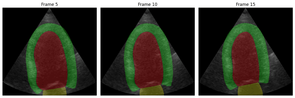
As you can see, the model can segment the heart components correctly:
- Red Region: Likely the left ventricle cavity, where blood fills during diastole and is pumped out during systole.
- Green Region: Appears to be the myocardium – the muscular wall of the left ventricle.
- Yellow Region: Probably the left ventricular outflow tract (LVOT) or part of the mitral valve apparatus, depending on the specific anatomical view.
So long, right! We have provided the notebook versions of these scripts, which you can run easily on the flow.
PS: You can download all the notebooks in the Download Code button; these are slightly modified and adapted from the original MedSAM2 repository.
Now let’s summarize what we have learned so far!
TL;DR
- The Challenge in Medical Imaging – Doctors often manually draw boundaries on thousands of scan slices, a time-consuming and labor-intensive process.
- Why Segmentation Matters – It’s the entry point for AI in hospitals, helping with surgery preparation, ER diagnosis, and powering downstream tools like tumor models and 3D printing.
- What is MedSAM2 – A powerful “Segment Anything” model adapted for 3D medical images and real-time videos. It needs only one box or click to work across modalities.
- Architecture Upgrades – Combines the speed of SAM2 with short-term memory blocks for 3D awareness and temporal consistency in video.
- Training on Massive Multi-Modal Medical Data – Trained on 450k+ 3D scans and 76k+ echo/endoscopy frames, with human-in-the-loop refinement for accuracy.
- Code Workflow and Performance – From CT scans to echo videos, MedSAM2 performs fast, high-accuracy segmentation using a consistent, reproducible PyTorch pipeline.
- Real Impact – Up to 90% reduction in manual segmentation time, real-time echo tracking, and generalizability across organs and modalities.
Conclusion
MedSAM2 represents a significant leap forward in medical imaging AI, simplifying 3D and video segmentation with a single prompt, model, and real-time performance. It builds on years of progress in computer vision and applies it directly to the most urgent challenges in healthcare. Faster diagnosis, less manual work, and broader access to precision tools are no longer futuristic goals – they’re here now.
See you in the next blog, bye!
References
MedSAM2: Segment Anything in 3D Medical Images and Videos
AI in Medical Imaging Market Size
Revolutionizing Medical Imaging with Semantic Segmentation
Segment anything in medical images







100K+ Learners
Join Free OpenCV Bootcamp3 Hours of Learning