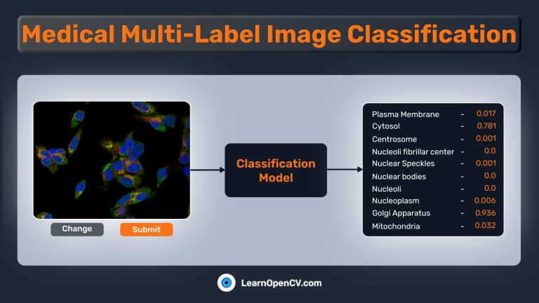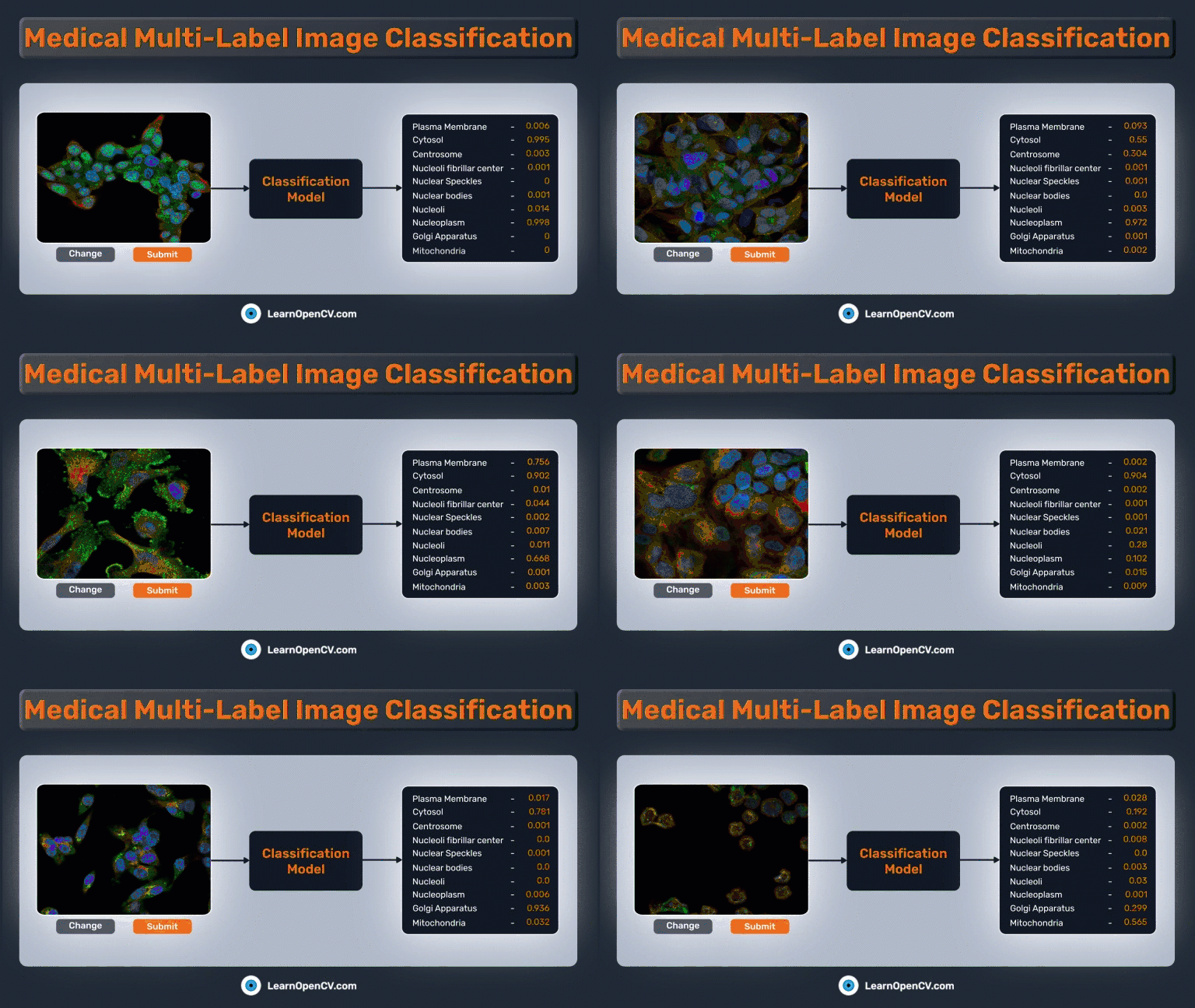
Medical Multi-label Classification With PyTorch & Lightning

medical_multi-label_feature_GIF – LearnOpenCV

In the pivotal field of medical diagnostics, swift and accurate image classification plays a crucial role in aiding healthcare professionals’ decision-making. The advent of deep learning, coupled with potent frameworks like PyTorch, has made it possible to apply leading-edge models to tackle complex tasks such as medical multi-label image classification. In this demonstration, we will employ a subset of the “Human Protein Atlas Image Classification” dataset from Kaggle to showcase these concepts and tackle a related challenge.

We will explore the use of PyTorch in conjunction with the widely-used pytorch-lightning library to fine-tune the pre-trained EfficientNetv2 model from torchvision. Additionally, we will demonstrate how to create a Gradio application for model inference.

Grid of sample images from medical multi-label dataset.

Note: This blog post is designed for readers familiar with Convolutional Neural Networks (CNNs), PyTorch basics, and multi-class classification who want to learn about multi-label classification. It provides insights into the differences between multi-class and multi-label classification, explores the differences, and offers valuable resources to enhance understanding in this specific area.

What is Multi-Label Image Classification? A Quick Recap
Human Protein Atlas Dataset
Building The Medical Multi-Label Image Classification Pipeline
Hyperparameters For Medical Multi-Label Project
Medical Multi-Label Dataset Preparation
Loading Pretrained Models From Torchvision
Creating A Custom LightningModule Class
Begin Training
Inference
Create a Gradio App For Image Classification
Summary

What is Multi-Label Image Classification? A Quick Recap

We can easily categorize any learning-based algorithm as a generative or discriminative model. By definition, “Classification” refers to the process of categorizing or grouping objects, data, or instances into predefined classes or categories based on their characteristics or features. It is a fundamental task in machine learning and data mining, where the goal is to develop a model or algorithm that can automatically assign new, unseen instances to one of the predefined classes.

Difference between binary, multi-class and multi-label classficiation.

Source: https://www.microsoft.com/en-us/research/uploads/prod/2017/12/40250.jpg

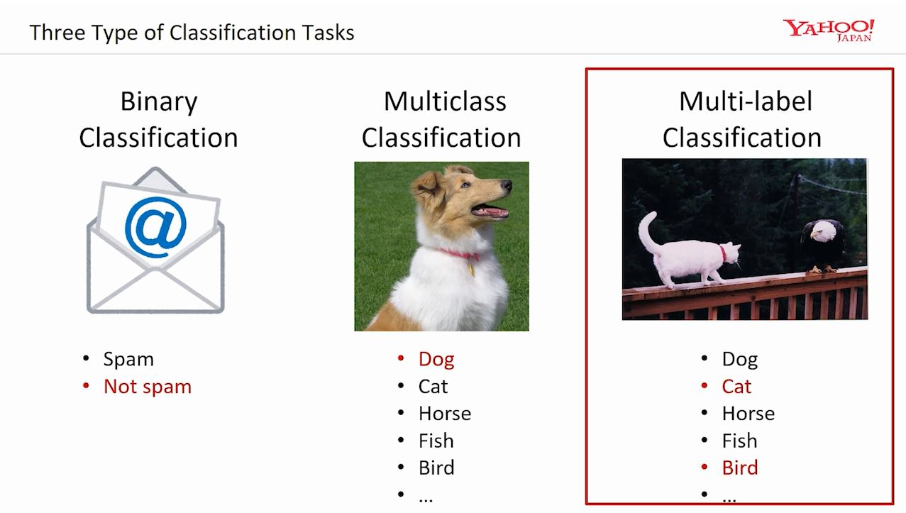
Binary Image Classification

It’s like teaching a computer to answer a simple question about pictures. We show it many pictures and ask, “Is there something specific in this picture?” The computer looks for clues and patterns in the pictures to figure out the answer. When we present it with another picture, it uses what it has learned to answer “yes” or “no” if a specific thing appears.

Multi-Class Image Classification

Multi-class image classification is a task where a computer is trained to recognize and categorize images into more than two classes or categories. It’s like teaching a computer to play a game of “Guess Who?” with pictures. We show it different pictures of animals and objects and ask, “Is it a cat, a dog, a panda, or something else?” The computer looks at the pictures and learns the specific things about each animal or object to make the correct guess. Subsequently, when we show it a new picture, it uses what it learned to guess which animal or object it is from the given choices.

Multi-Label Image Classification

Multi-label image classification is a task where a computer is trained to recognize and assign multiple labels or tags to an image. Instead of assigning a single category to an image, as in the case of multi-class classification, multi-label classification allows for the possibility of multiple objects, attributes, or concepts simultaneously being present in an image. For example, an image could be labeled with tags such as “cat,” “tree,” and “sunny.” The computer learns to identify and associate different labels with specific regions, objects, or attributes within an image. This type of classification is particularly useful when dealing with complex scenes or images where multiple objects or attributes coexist, providing a more detailed and comprehensive understanding of the image content. Basically, it’s like the computer can recognize and describe multiple aspects of an image, like a tagger identifying and labeling various objects.

Difference Between Multi-Class & Multi-Label Image Classification

The difference in targets between multi-class and multi-label image classification.

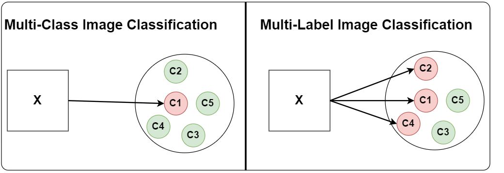
Multi-Class Classification suffers from the constraint of being able to associate only one class with each image. Still, it works as long as

Each image generally contains only one class.
The presence of other object classes does not matter.

On the other hand, Multi-Label Image Classification is formulated in a way that each image can be associated with multiple classes.

Each image can have multiple objects.
And each image can belong to a different category.

Model Output Logits & Loss Function

Next, we will see the difference between multi-class and multi-label image classification with respect to target vectors and the activation function used for the final layer.

Multi-Class Image Classification
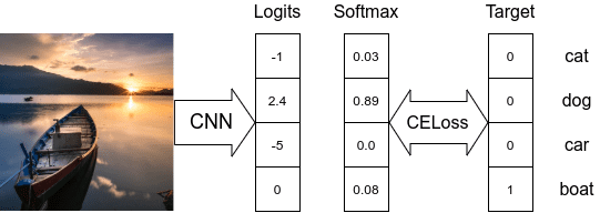
- While dealing with multi-class classification problems, a classifier assumes that each sample is assigned to one and only one label.
- The output target is only a single class.
- The target Y can be either the class id integer or a one-hot encoded vector. In PyTorch, the nn.CrossEntropyLoss(...) class takes the class Id of the ground truth.

 Multi-Label Image Classification
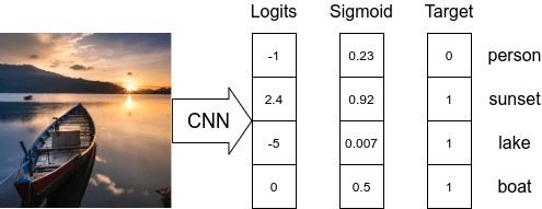
  By definition, we cannot use a one-hot encoded vector or a single integer class id to represent an output for multi-label classification.
 The target vector needs to be represented as an array of class IDs or (more generally) a vector of 0’s except 1’s at index positions related to the current labels. This can be performed using scikit-learn’s MultiLabelBinarizer. We have defined a custom function encode_label(...) to help with the conversion.
 The Sigmoid activation function is applied to every node in the final layer to normalize the node logits value between 0 and 1.
 As each model node can be considered as output, we need to apply Binary Cross-Entropy loss at each node and then reduce the loss value of each node to calculate the final loss value.
 In PyTorch, to calculate loss, we can use nn.BCELoss(...) class takes in sigmoid normalized model logits as input values or nn.BCEWithLogitsLoss(...) class which works with the model’s logits.
 Usually, a threshold value is used to select the output node as a valid prediction. If the sigmoid output is above the threshold, then the class id corresponding node is given as output.

  
 Human Protein Atlas Dataset
 In this project, we will use a subset of the original Human Protein Atlas Image Classification challenge dataset. The original dataset has 28 classes, with certain classes being abundant while some only have a fraction available.
  
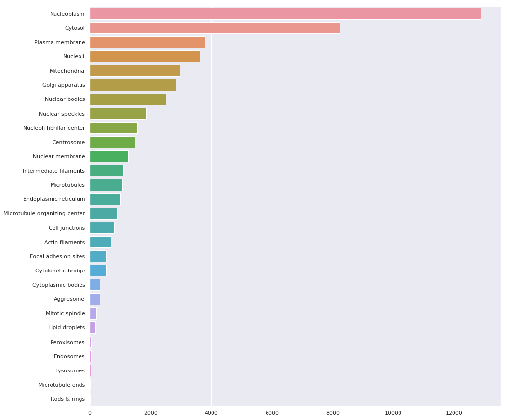
 Source: https://www.kaggle.com/code/allunia/protein-atlas-exploration-and-baseline
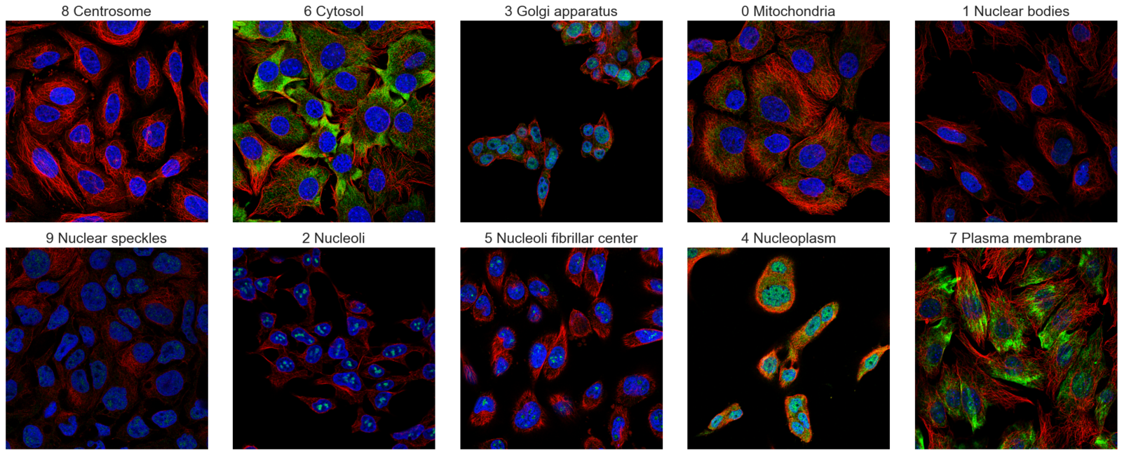
 As this post is geared more towards the theory + code behind multi-label image classification problems, we will use the subset dataset in the Zero to GANs – Human Protein Classification. The dataset was created from the training set of the Human protein atlas dataset, and the number of classes was limited to the top 10 most available classes.
 labels = {
    0: 'Mitochondria',
    1: 'Nuclear bodies',
    2: 'Nucleoli',
    3: 'Golgi apparatus',
    4: 'Nucleoplasm',
    5: 'Nucleoli fibrillar center',
    6: 'Cytosol',
    7: 'Plasma membrane',
    8: 'Centrosome',
    9: 'Nuclear speckles'
}
  
 The classes are still imbalanced, but we can work with this:
 
 import pandas as pd
from itertools import chain
from collections import Counter

data_df = pd.read_csv(DatasetConfig.TRAIN_CSV) # path to the train.csv file


all_labels = list(chain.from_iterable([i.strip().split(" ") for i in data_df["Label"].values]))
c_val = Counter(all_labels)

n_keys = c_val.keys()
max_idx = max(n_keys)

counts = pd.DataFrame(
    {
        
        "Label": [labels[int(key)] for key in c_val.keys()],
        "Count": [val for val in c_val.values()],
    }
)

rev_label2id = {value: key for key, value in labels.items()}
counts["Class ID"]  = [rev_label2id[label] for label in counts["Label"]]
counts = counts.set_index("Class ID")

counts = counts.sort_values(by="Count", ascending=False)
counts.style.background_gradient(cmap="Reds")
  
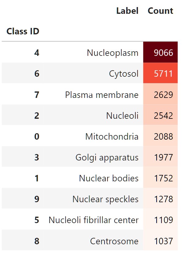
 We can also plot class counts as a bar graph using Seaborn:
 import seaborn as sns

sns.set_palette(sns.color_palette("rocket_r"))
plt.figure(figsize=(10,5))
sns.barplot(y=counts["Label"].values, x=counts["Count"].values, order=counts["Label"].values);
  
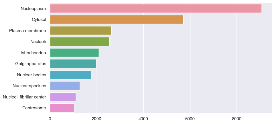
 In the dataset, there are 19236 images with their labels available. We will split the dataset into a 90:10 ratio to create a training and validation set during training.
 Here’s another set of images to illustrate that we do indeed have a multi-label image dataset.
  
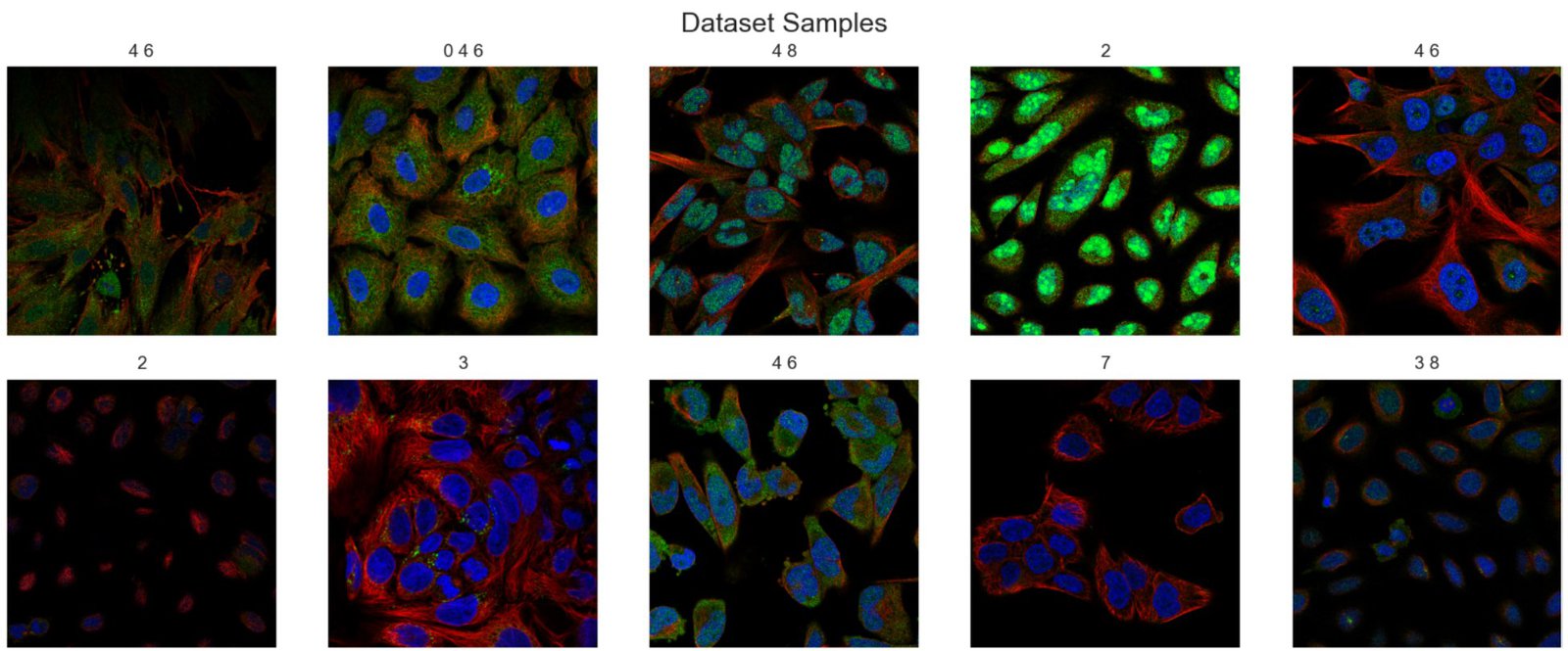
 Note: You can either download the datasets manually, upload/move them to your work machine or use the data downloading code we have added in Lightning’s (pytorch-lightning) LightningDataModule class to download it automatically from Kaggle.
 Building The Medical Multi-Label Image Classification Pipeline
 Starting here, we will focus solely on coding and building the pipeline using pytorch-lightning. We are using lightning because it removes all the boilerplate code one must write in every project. Some of the benefits we experienced when using it for the project are:
  Better code structuring.
 No need to write additional code for checkpoints or learning rate monitoring.
 Easily train with a distributed setting. For e.g., We trained the model on a 2x 3090 GPU system on the cloud to speed up training.
 No need to write training loops or additional mixed-precision training code.
 No need to write custom tensorboard logging code.
 
 The entire pipeline consists of 3 main components.
  Creating a custom ProteinDataModule inherited from LightningDataModule class. This class will contain all the required code related to downloading & creating datasets and dataloaders.
 Initializing a pre-trained model. The model can be loaded from anywhere. We use the pre-trained EfficientNetv2-small model trained on (384×384) image size for this project.
 Creating a custom ProteinModel class inherited from LightningModule class. This class will hold all the code regarding training, evaluation, initializing optimizers, and any learning rate schedulers.
 
   Download Code To easily follow along this tutorial, please download code by clicking on the button below. It's FREE! Download Code
 
         
 
    Click here to download the source code to this post  
 
 
 
 
 
 
 Importing Required Libraries
 Before we begin the coding part, we need to ensure we have all the required libraries installed. Assuming you have PyTorch preinstalled, to install the additional required libraries, execute the following
 pip install -qqqU kaggle torchinfo lightning==2.0.1 torchmetrics==1.0.0 gradio
pip install -qqq opencv-contrib-python tqdm tensorboard scikit-learn seaborn
 Next, we will import all the necessary functions and classes for the project.
 import os
import shutil
import warnings
import platform
from glob import glob
from itertools import chain
from collections import Counter
from dataclasses import dataclass

import numpy as np
import pandas as pd
import seaborn as sns
from PIL import Image
import matplotlib.pyplot as plt
# from sklearn.utils.class_weight import compute_class_weight

# Next, we have our usual torch and torchvision imports.
import torch
import torch.nn as nn
import torch.optim as optim
from torch.utils.data import Dataset, DataLoader

import torchvision
import torchvision.transforms as TF
from torchvision.utils import make_grid
from torchvision.ops import sigmoid_focal_loss

# Importing lighting along with a built-in callback it provides.
import lightning.pytorch as pl
from lightning.pytorch.callbacks import LearningRateMonitor, ModelCheckpoint

# Importing torchmetrics modular and functional evaluation implementations.
from torchmetrics import MeanMetric
from torchmetrics.classification import MultilabelF1Score

# To print model summary.
from torchinfo import summary
 Hyperparameters For Medical Multi-Label Project
 First, we define the root location where we want to download the dataset. The location for the rest of the folders, such as training and test set images, will use this location as the base path.
 # Set root path where dataset will be downloaded. 
# Every other path to the folder or files in the datasets, 
# will have this as it's root

ROOT_DATASET_PATH = os.path.join(os.getcwd(), "datasets")
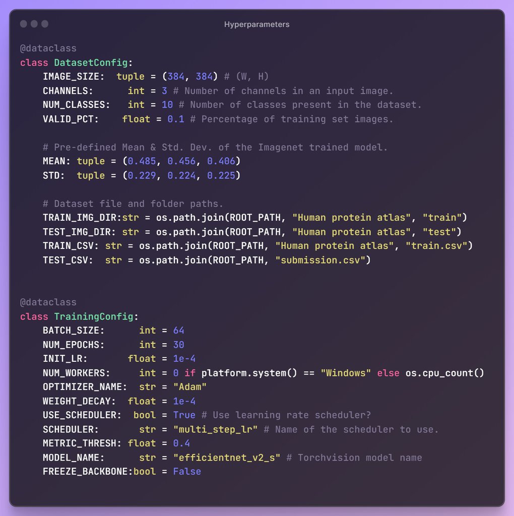
 Next, we are defining two classes. 
  DatasetConfig – A class that holds all the hyperparameters we will use for the processing of images. It contains the following information:  Image size to use.
 Number of classes present in the dataset,
 Percentage of the training set images to use for validation.
 The mean and standard deviation to use for image normalization.
 Path to training and test set images along with the train.csv, which contains label id information for each image.
 
 
 TrainingConfig –  A class that holds all the hyperparameters we will use for training and evaluation.  It contains the following information:  Batch size.
 Initial learning rate.
 The number of epochs to train the model.
 The number of workers to use for data loading.
 Model, optimizer & learning rate scheduler-related configurations.
 The threshold during metric calculation.
 To freeze the backbone model or not. If true, only the final classifier layer will be trained. Here, we found as the dataset domain is very different than the one the model is trained on, so we will train the entire model along with the final classification layer together from the start.
 
 
 
 You can define anything you want within this class. The goal is to have all the necessary constants defined in one place.
  
 Medical Multi-Label Dataset Preparation
 Before we begin writing our custom LightningModule class, we need additional helper functions and classes for the following tasks.
 We need to define three helper functions and one custom PyTorch Dataset class:
 A) encode_label(...) : This function converts labels in string format into a vector of 0’s and 1’s depending on the provided label. For example, “1 3 5” → [0, 1, 0, 1, 0, 1, 0, 0, 0, 0].
 def encode_label(label: list, num_classes=10):
    """This functions converts labels into one-hot encoding"""

    target = torch.zeros(num_classes)
    for l in str(label).split(" "):
        target[int(l)] = 1.0
    return target
 B) decode_target(...):  This function converts the model’s prediction from a vector of probabilities to a string of integers (“1 4 5”) or their string (class names) representations.
 def decode_target(
    target: list,
    text_labels: bool = False,
    threshold: float = 0.4,
    cls_labels: dict = None,
):
    """This function converts the labels from
    probablities to outputs or string representations
    """

    result = []
    for i, x in enumerate(target):
        if x >= threshold:
            if text_labels:
                result.append(cls_labels[i] + "(" + str(i) + ")")
            else:
                result.append(str(i))
    return " ".join(result)
 C) denormalize(...): This function denormalizes the image tensors and clip values between 0 and 1. It is helpful during image visualizations.
 def denormalize(tensors, *, mean, std):
    """Denormalizes image tensors using mean and std provided
    and clip values between 0 and 1"""

    for c in range(DatasetConfig.CHANNELS):
        tensors[:, c, :, :].mul_(std[c]).add_(mean[c])

    return torch.clamp(tensors, min=0.0, max=1.0)
 D) HumanProteinDataset: This is a custom PyTorch Dataset class designed to load each set’s images and labels (if available). The PyTorch “Dataset” class is essential for efficient and organized data handling in machine learning tasks. It provides a standardized interface to load and preprocess data samples from various sources. Encapsulating the dataset into a single object simplifies data management. It enables seamless integration with other PyTorch components like data loaders and models.
 class HumanProteinDataset(Dataset):
    """
    Parse raw data to form a Dataset of (X, y).
    """

    def __init__(self, *, df, root_dir, img_size, transforms=None, is_test=False):
        self.df = df
        self.root_dir = root_dir
        self.img_size = img_size
        self.transforms = transforms
        self.is_test = is_test

    def __len__(self):
        return len(self.df)

    def __getitem__(self, idx):
        row = self.df.loc[idx]
        img_id = row["Image"]
        img_fname = self.root_dir + os.sep + str(img_id) + ".png"
        
        img = Image.open(img_fname).convert("RGB")
        img = img.resize(self.img_size, resample=3)
        img = self.transforms(img)
        
        if self.is_test:
            return img, img_id
    
        return img, encode_label(row["Label"])
 Custom LightningDataModule Class To Load The Medical Multi-Label Dataset
 The first primary class is the ProteinDataModule which inherits from Lightning’s LightningDataModule class. The custom class encapsulates the following steps:
  Download the dataset from Kaggle.
 Create train and validation splits.
 Create a Dataset class object for each split with appropriate transformations.
 Create DataLoader objects for each split.
 
 The class methods are defined to do the following tasks:
  prepare_data(..): This method is used for data preparation, like downloading and one-time preprocessing with the dataset. When training on a distributed GPU, this will be called from a single GPU.
 setup(...):  When you want to perform data operations on every GPU, this method is apt for it will call from every GPU. For example, perform train/val/test splits.
 train_dataloader(...): This method returns the train dataloader.
 val_dataloader(...): This method returns validation dataloader(s).
 test_dataloader(...):  This method returns test dataloader(s).
 
 
 Note: Please ensure that your Kaggle credential files kaggle.json is either available in the root user path.
 # Get kaggle user folder location in your machine.
KAGGLE_DIR = os.path.join(os.path.expanduser("~"), ".kaggle")
print(KAGGLE_DIR)
 You can download your credentials (JSON) file from your Kaggle account if it’s available. Go to your Kaggle Profile >> the Account tabs >> Click Create New Token. Save the file in the current working directory, and the prepare_data(..) method will automatically move the file to the required location for you.
 
 class ProteinDataModule(pl.LightningDataModule):
    def __init__(
        self,
        *,
        num_classes=10,
        valid_pct=0.1,
        resize_to=(384, 384),
        batch_size=32,
        num_workers=0,
        pin_memory=False,
        shuffle_validation=False,
    ):
        super().__init__()

        self.num_classes = num_classes
        self.valid_pct = valid_pct
        self.resize_to = resize_to
        self.batch_size = batch_size
        self.num_workers = num_workers
        self.pin_memory = pin_memory
        self.shuffle_validation = shuffle_validation

        self.train_tfs = TF.Compose(
            [
                TF.RandomAffine(
                    degrees=40,
                    translate=(0.01, 0.12),
                    shear=0.05,
                ),
                TF.RandomHorizontalFlip(),
                TF.RandomVerticalFlip(),
                TF.ToTensor(),
                TF.Normalize(DatasetConfig.MEAN, DatasetConfig.STD, inplace=True),
                TF.RandomErasing(inplace=True),
            ]
        )

        self.valid_tfs = TF.Compose(
            [
                TF.ToTensor(),
                TF.Normalize(DatasetConfig.MEAN, DatasetConfig.STD, inplace=True),
            ]
        )
        self.test_tfs = self.valid_tfs


    def prepare_data(self):
        # Download dataset.
        if not os.path.exists(os.path.join(DatasetConfig.TRAIN_CSV)):
            KAGGLE_DIR = os.path.join(os.path.expanduser("~"), ".kaggle")
            KAGGLE_JSON_PATH = os.path.join(KAGGLE_DIR, "kaggle.json")

            if not os.path.exists(KAGGLE_JSON_PATH):
                os.makedirs(KAGGLE_DIR, exist_ok=True)
                shutil.copyfile("kaggle.json", KAGGLE_JSON_PATH)
                os.chmod(KAGGLE_JSON_PATH, 0o600)

            # print("Downloading 512x512 sized dataset...", end="")
            # !kaggle datasets download -q aakashns/jovian-pytorch-z2g -p datasets --unzip

            print("Downloading 384x384 sized dataset...", end="")
            !kaggle datasets download -q learnopencvblog/human-protein-atlas-384x384 -p {ROOT_PATH} --unzip
            print("Done")

    def setup(self, stage=None):
        np.random.seed(42)
        data_df = pd.read_csv(DatasetConfig.TRAIN_CSV)
        msk = np.random.rand(len(data_df)) < (1.0 - self.valid_pct)
        train_df = data_df[msk].reset_index()
        valid_df = data_df[~msk].reset_index()

        # train_labels = list(chain.from_iterable([i.strip().split(" ") for i in train_df["Label"].values]))
        # class_weights = compute_class_weight("balanced", classes=list(range(self.num_classes)), 
        #                                      y=[int(i) for i in train_labels])
        # self.class_weights = torch.tensor(class_weights)

        img_size = DatasetConfig.IMAGE_SIZE
        self.train_ds = HumanProteinDataset(
            df=train_df, img_size=img_size, root_dir=DatasetConfig.TRAIN_IMG_DIR, transforms=self.train_tfs
        )

        self.valid_ds = HumanProteinDataset(
            df=valid_df, img_size=img_size, root_dir=DatasetConfig.TRAIN_IMG_DIR, transforms=self.valid_tfs
        )

        test_df = pd.read_csv(DatasetConfig.TEST_CSV)
        self.test_ds = HumanProteinDataset(
            df=test_df, img_size=img_size, root_dir=DatasetConfig.TEST_IMG_DIR, transforms=self.test_tfs, is_test=True
        )

        print(f"Number of images :: Training: {len(self.train_ds)}, Validation: {len(self.valid_ds)}, Testing: {len(self.test_ds)}\n")

    def train_dataloader(self):
        # Create a train dataloader.
        train_loader = DataLoader(
            self.train_ds, batch_size=self.batch_size, pin_memory=self.pin_memory, shuffle=True, num_workers=self.num_workers
        )
        return train_loader

    def val_dataloader(self):
        # Create validation dataloader object.
        valid_loader = DataLoader(
            self.valid_ds, batch_size=self.batch_size, pin_memory=self.pin_memory, 
            shuffle=self.shuffle_validation, num_workers=self.num_workers
        )
        return valid_loader

    def test_dataloader(self):
        # Create test dataloader object.
        test_loader = DataLoader(
            self.test_ds, batch_size=self.batch_size, pin_memory=self.pin_memory, shuffle=False, num_workers=self.num_workers
        )
        return test_loader
 Loading Pretrained Models From Torchvision
 In this section, we define a helper function capable of loading any classification model available in Torchvision. All you need to do is pass the following:
  The correct model_name. For e.g. “resnet50” for the ResNet-50 model, “mobilenet_v3_large” for the MobileNetV3-Large model.
 num_classes: The number of nodes in the output layer of the model.
 freeze_backbone: Whether to freeze the rest of the parameters of the model.
 
 def get_model(model_name: str, num_classes: int, freeze_backbone: bool= True):
    """A helper function to load and prepare any classification model 
    available in Torchvision for transfer learning or fine-tuning."""
    
    model = getattr(torchvision.models, model_name)(weights="DEFAULT")
    
    if freeze_backbone:
        # Set all layer to be non-trainable
        for param in model.parameters():
            param.requires_grad = False
        
    model_childrens = [name for name, _ in model.named_children()]

    try:
        final_layer_in_features = getattr(model, f"{model_childrens[-1]}")[-1].in_features
    except Exception as e:
        final_layer_in_features = getattr(model, f"{model_childrens[-1]}").in_features

    new_output_layer = nn.Linear(
        in_features=final_layer_in_features, 
        out_features=num_classes
    )
    
    try:
        getattr(model, f"{model_childrens[-1]}")[-1] = new_output_layer
    except:
        setattr(model, model_childrens[-1], new_output_layer)
    
    return model
 Function usage example:
 model = get_model(
    model_name=TrainingConfig.MODEL_NAME, 
    num_classes=DatasetConfig.NUM_CLASSES,
    freeze_backbone=False,
)

summary(
    model, 
    input_size=(1, DatasetConfig.CHANNELS, *DatasetConfig.IMAGE_SIZE[::-1]), 
    depth=2, 
    device="cpu", 
    col_names=["output_size", "num_params", "trainable"]
)
 Model summary:
 ==================================================================================================================================
Layer (type:depth-idx)                                  Output Shape              Param #                   Trainable
==================================================================================================================================
EfficientNet                                            [1, 10]                   --                        True
├─Sequential: 1-1                                       [1, 1280, 12, 12]         --                        True
│    └─Conv2dNormActivation: 2-1                        [1, 24, 192, 192]         696                       True
│    └─Sequential: 2-2                                  [1, 24, 192, 192]         10,464                    True
│    └─Sequential: 2-3                                  [1, 48, 96, 96]           303,552                   True
│    └─Sequential: 2-4                                  [1, 64, 48, 48]           589,184                   True
│    └─Sequential: 2-5                                  [1, 128, 24, 24]          917,680                   True
│    └─Sequential: 2-6                                  [1, 160, 24, 24]          3,463,840                 True
│    └─Sequential: 2-7                                  [1, 256, 12, 12]          14,561,832                True
│    └─Conv2dNormActivation: 2-8                        [1, 1280, 12, 12]         330,240                   True
├─AdaptiveAvgPool2d: 1-2                                [1, 1280, 1, 1]           --                        --
├─Sequential: 1-3                                       [1, 10]                   --                        True
│    └─Dropout: 2-9                                     [1, 1280]                 --                        --
│    └─Linear: 2-10                                     [1, 10]                   12,810                    True
==================================================================================================================================
Total params: 20,190,298
Trainable params: 20,190,298
Non-trainable params: 0
Total mult-adds (G): 8.36
==================================================================================================================================
Input size (MB): 1.77
Forward/backward pass size (MB): 571.97
Params size (MB): 80.76
Estimated Total Size (MB): 654.50
==================================================================================================================================
 Creating A Custom LightningModule Class
 The final custom class we need to define is the ProteinModel class which inherits from the LightningModule class. The  LightningModule class helps to properly organize the PyTorch code into separate sections for training and evaluation. 
 #No Action Method
1 Initialization __init__(...)
2 Training Loop training_step(...)
3 Validation Loop validation_step(...)
4 Testing Loop test_step(...)
5 Prediction Loop predict_step(...)
6 Initialize Optimizer & schedulers configure_optimizers(...)
 Scoring Mechanism
 Before writing our custom class, it’s crucial to select an appropriate evaluation metric. Due to the imbalanced nature of our dataset, relying on “accuracy” alone can be misleading. Accuracy measures the proportion of correct predictions out of all predictions made by the model.
 
      
 In an imbalanced dataset, where the number of instances of one class greatly outnumbers the other, a model could achieve high accuracy simply by predicting the majority class all the time. In such cases, the F1-score is a commonly used metric. It is the harmonic mean of precision and recall- two fundamental measures of a model’s effectiveness. Precision measures how many of the predicted positive instances are actually positive, while recall measures how many actual positive instances were correctly predicted by the model. F1 score is particularly useful when the data is imbalanced, that is when the cost of false positives and false negatives are significantly different. 
 To calculate the F1 score for the medical multi-label classification task, we will use the MultilabelF1Score class from the torchmetrics library and the “macro” average reduction method.
 “Macro” average refers to a method of calculating average performance in multiclass or multilabel classification problems, which treats all classes equally.
 
 To summarize, for the medical multi-label dataset, we are using the following:
  Pre-trained efficientnet_v2_s model.
 BCEWithLogitsLoss loss.
 MultilabelF1Score as the evaluation metric.
 Adam optimizer.
 MultiStepLr LR scheduler that decays the learning rate at the halfway point in training.
 
 
 class ProteinModel(pl.LightningModule):
    def __init__(
        self,
        model_name: str,
        num_classes: int = 10,
        freeze_backbone: bool = False,
        init_lr: float = 0.001,
        optimizer_name: str = "Adam",
        weight_decay: float = 1e-4,
        use_scheduler: bool = False,
        f1_metric_threshold: float = 0.4,
    ):
        super().__init__()

        # Save the arguments as hyperparameters.
        self.save_hyperparameters()

        # Loading model using the function defined above.
        self.model = get_model(
            model_name=self.hparams.model_name,
            num_classes=self.hparams.num_classes,
            freeze_backbone=self.hparams.freeze_backbone,
        )

        # Intialize loss class.
        self.loss_fn = nn.BCEWithLogitsLoss()

        # Initializing the required metric objects.
        self.mean_train_loss = MeanMetric()
        self.mean_train_f1   = MultilabelF1Score(num_labels=self.hparams.num_classes, 
                                                 average="macro", threshold=self.hparams.f1_metric_threshold)
        self.mean_valid_loss = MeanMetric()
        self.mean_valid_f1   = MultilabelF1Score(num_labels=self.hparams.num_classes, 
                                                 average="macro", threshold=self.hparams.f1_metric_threshold)

    def forward(self, x):
        return self.model(x)

    def training_step(self, batch, *args, **kwargs):
        data, target = batch
        logits = self(data)
        loss = self.loss_fn(logits, target)
        
        self.mean_train_loss(loss, weight=data.shape[0])
        self.mean_train_f1(logits, target)

        self.log("train/batch_loss", self.mean_train_loss, prog_bar=True)
        self.log("train/batch_f1",   self.mean_train_f1,   prog_bar=True)
        return loss

    def on_train_epoch_end(self):
        # Computing and logging the training mean loss & mean f1.
        self.log("train/loss", self.mean_train_loss, prog_bar=True)
        self.log("train/f1",   self.mean_train_f1,   prog_bar=True)
        self.log("step", self.current_epoch)

    def validation_step(self, batch, *args, **kwargs):
        data, target = batch  # Unpacking validation dataloader tuple
        logits = self(data)
        loss = self.loss_fn(logits, target)
        
        self.mean_valid_loss.update(loss, weight=data.shape[0])
        self.mean_valid_f1.update(logits, target)

    def on_validation_epoch_end(self):
        # Computing and logging the validation mean loss & mean f1.
        self.log("valid/loss", self.mean_valid_loss, prog_bar=True)
        self.log("valid/f1",   self.mean_valid_f1,   prog_bar=True)
        self.log("step", self.current_epoch)

    def configure_optimizers(self):
        optimizer = getattr(torch.optim, self.hparams.optimizer_name)(
            filter(lambda p: p.requires_grad, self.model.parameters()),
            lr=self.hparams.init_lr,
            weight_decay=self.hparams.weight_decay,
        )

        if self.hparams.use_scheduler:
            lr_scheduler = torch.optim.lr_scheduler.MultiStepLR(
                optimizer,
                milestones=[self.trainer.max_epochs // 2,],
                gamma=0.1,
            )

            # The lr_scheduler_config is a dictionary that contains the scheduler
            # and its associated configuration.
            lr_scheduler_config = {
                "scheduler": lr_scheduler,
                "interval": "epoch",
                "name": "multi_step_lr",
            }
            return {"optimizer": optimizer, "lr_scheduler": lr_scheduler_config}

        else:
            return optimizer
 Begin Training
 Once we have organized the LightningModule and LightningDataModule classes, utilizing the Trainer class automates the remaining tasks effortlessly. The Trainer offers a range of valuable deep learning training functionalities, such as mixed-precision training, distributed training, deterministic training, profiling, gradient accumulation, batch overfitting, and more. Implementing these functionalities correctly can be time-consuming, but it becomes a swift process with the Trainer class.
 By initializing our ProteinModel and ProteinDataModule classes and passing them to the .fit(...) method of the Trainer class instance, we can promptly commence training. This streamlined approach eliminates the need for manual implementation of various training aspects, providing convenience and efficiency.
 # Seed everything for reproducibility.
pl.seed_everything(42, workers=True)

model = ProteinModel(
    model_name=TrainingConfig.MODEL_NAME,
    num_classes=DatasetConfig.NUM_CLASSES,
    freeze_backbone=TrainingConfig.FREEZE_BACKBONE,
    init_lr=TrainingConfig.INIT_LR,
    optimizer_name=TrainingConfig.OPTIMIZER_NAME,
    weight_decay=TrainingConfig.WEIGHT_DECAY,
    use_scheduler=TrainingConfig.USE_SCHEDULER,
    f1_metric_threshold=TrainingConfig.METRIC_THRESH,
)

data_module = ProteinDataModule(
    num_classes=DatasetConfig.NUM_CLASSES,
    valid_pct=DatasetConfig.VALID_PCT,
    resize_to=DatasetConfig.IMAGE_SIZE,
    batch_size=TrainingConfig.BATCH_SIZE,
    num_workers=TrainingConfig.NUM_WORKERS,
    pin_memory=torch.cuda.is_available(),
)

# Creating ModelCheckpoint callback.
# Checkpoints by default will be saved in Trainer - default_root_dir which is "lightning_logs".
model_checkpoint = ModelCheckpoint(
    monitor="valid/f1",
    mode="max",
    filename="ckpt_{epoch:03d}-vloss_{valid/loss:.4f}_vf1_{valid/f1:.4f}", 
    auto_insert_metric_name=False,
)

# Creating a learning rate monitor callback which will be plotted/added in the default logger.
lr_rate_monitor = LearningRateMonitor(logging_interval="epoch")

# Initializing the Trainer class object.
# It uses 'Tensorboard' as its default logger.
trainer = pl.Trainer(
    accelerator="auto", # Auto select the best hardware accelerator available
    devices="auto", # Auto select available devices for the accelerator (For eg. mutiple GPUs)
    strategy="auto", # Auto select the distributed training strategy.
    max_epochs=TrainingConfig.NUM_EPOCHS, # Maximum number of epoch to train for.
    deterministic=True, # For deteministic and reproducible training.
    enable_model_summary=False, # Disable printing of model summary as we are using torchinfo.
    callbacks=[model_checkpoint, lr_rate_monitor],  # Declaring callbacks to use.
    precision="16", # Using Mixed Precision training.
    logger=True, # Auto generate TensorBoard logs.
)

# Start training
trainer.fit(model, data_module)

# Get path of the best saved model.
CKPT_PATH = model_checkpoint.best_model_path
 Inference
 To perform inference, first, we need to load the best checkpoint saved during training. We can do it simply by executing the following:
 CKPT_PATH = model_checkpoint.best_model_path
model = ProteinModel.load_from_checkpoint(CKPT_PATH)
 Next, we will evaluate the performance of the best-saved model on the validation set to assess its effectiveness.
 # Initialize trainer class for inference.
trainer = pl.Trainer(
    accelerator="gpu",
    devices=1,        
    enable_checkpointing=False,
    inference_mode=True,
)

# Run evaluation.
data_module.setup()
valid_loader = data_module.val_dataloader()
trainer.validate(model=model, dataloaders=valid_loader)
 The best validation set results are as follows:
 Validate metric Value
valid/f1 0.7903037071228027 
valid/loss 0.1759219616651535 
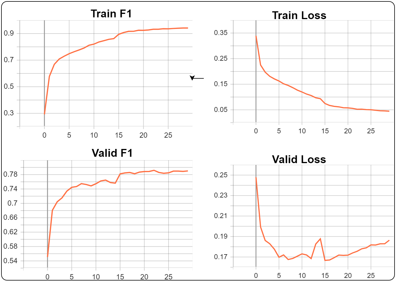
Training and Validation learning curves:
  
 You may notice that as that during the first 15 epochs, the validation set loss is decreasing, but once the LR is reduced (halfway point in training), the validation loss starts to increase. On the flip side, even though the validation loss is increasing, the validation F1 metric improves. This may occur because we have a low metric threshold value or the validation dataset is not diverse enough (diversity between classes and number of samples).
 To achieve better scores, you may check the competitions leaderboard page and refer to the solutions provided tried by the leaders—for example, multi-resolution training, focal loss, ensembling, and testing the model against different threshold values.
 Create a Gradio App For Image Classification
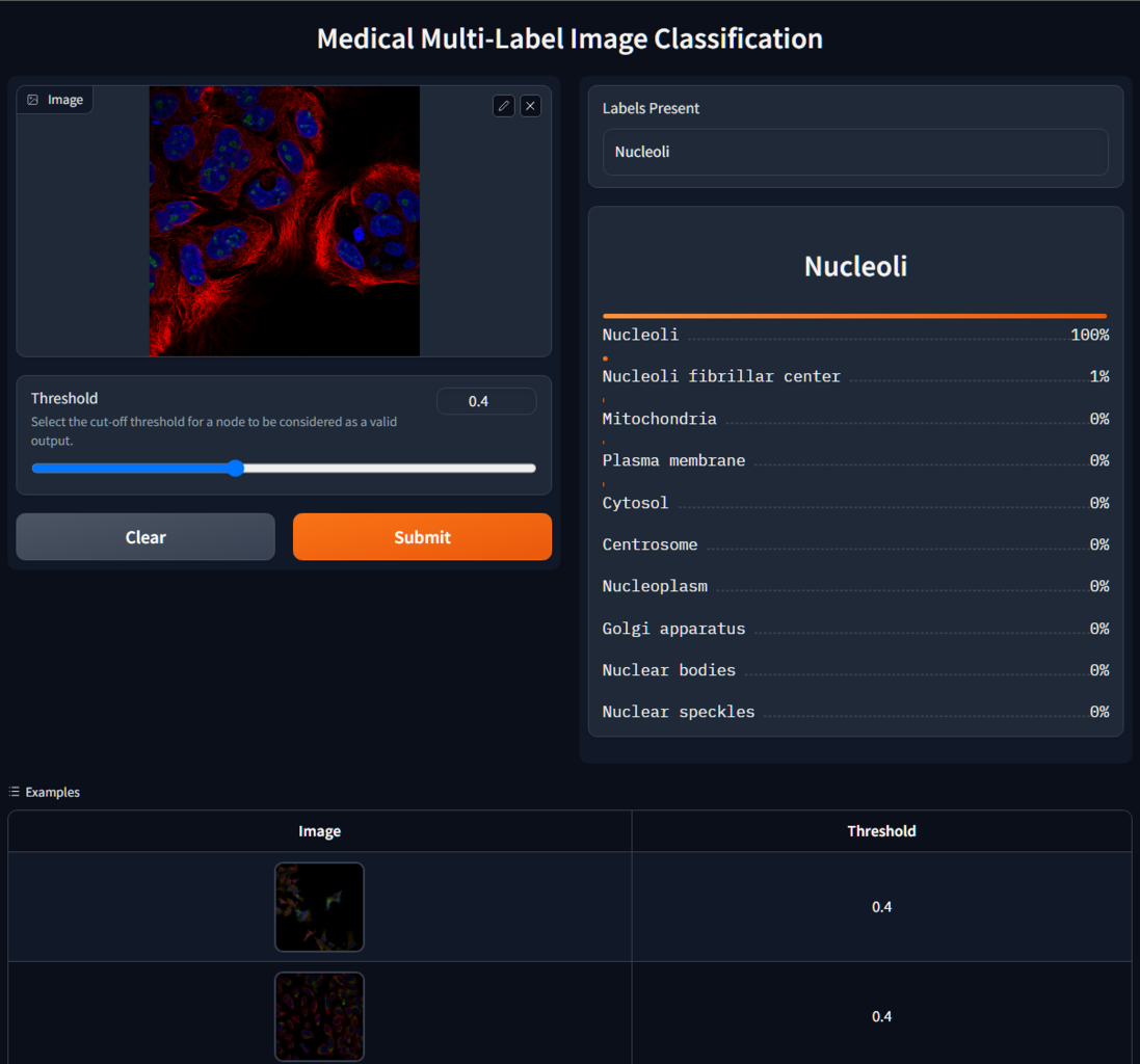
 As mentioned earlier, we’ll also create a UI using Gradio to perform predictions on any image. The Gradio app is straightforward and contains only 3 components:
  gr.Image(...) for providing images as input.
 gr.Slider(...) for providing a  custom threshold to select valid predictions.
 gr.Textbox(...) for printing the predicted class names.
 gr.Label(...) for showing a bar graph of each output node’s predicted probability.
 
 
 For demonstration purposes, we’ve also uploaded our Gradio app to HuggingFace. You can use the demo app here –> Medical Multi-Label Image Classification Gradio App
 All the files required can be accessed from here –> Gradio App Files
 
 The following code is part of an app.py file, which you can run by executing the command: 
 python app.py
 The majority of the code in the Python file remains the same. We use the existing TrainingConfig, DatasetConfig, get_model(...) function, and ProteinModel class. 
 The additional code needed is as follows:
 import gradio as gr

@torch.inference_mode()
def predict(input_image, threshold=0.4, model=None, preprocess_fn=None, device="cpu", idx2labels=None):
    input_tensor = preprocess_fn(input_image)
    input_tensor = input_tensor.unsqueeze(0).to(device)

    # Generate predictions
    output = model(input_tensor).cpu()

    probabilities = torch.sigmoid(output)[0].numpy().tolist()

    output_probs = dict()
    predicted_classes = []

    for idx, prob in enumerate(probabilities):
        output_probs[idx2labels[idx]] = prob
        if prob >= threshold:
            predicted_classes.append(idx2labels[idx])

    predicted_classes = "\n".join(predicted_classes)
    return predicted_classes, output_probs


if __name__ == "__main__":
    labels = {
        0: "Mitochondria",
        1: "Nuclear bodies",
        2: "Nucleoli",
        3: "Golgi apparatus",
        4: "Nucleoplasm",
        5: "Nucleoli fibrillar center",
        6: "Cytosol",
        7: "Plasma membrane",
        8: "Centrosome",
        9: "Nuclear speckles",
    }

    DEVICE = torch.device("cuda:0") if torch.cuda.is_available() else torch.device("cpu")
    CKPT_PATH = os.path.join(os.getcwd(), r"ckpt_022-vloss_0.1756_vf1_0.7919.ckpt")
    model = ProteinModel.load_from_checkpoint(CKPT_PATH)
    model.to(DEVICE)
    model.eval()
    _ = model(torch.randn(1, DatasetConfig.CHANNELS, *DatasetConfig.IMAGE_SIZE[::-1], device=DEVICE))

    preprocess = TF.Compose(
        [
            TF.Resize(size=DatasetConfig.IMAGE_SIZE[::-1]),
            TF.ToTensor(),
            TF.Normalize(DatasetConfig.MEAN, DatasetConfig.STD, inplace=True),
        ]
    )

    images_dir = glob(os.path.join(os.getcwd(), "samples") + os.sep + "*.png")
    examples = [[i, TrainingConfig.METRIC_THRESH] for i in np.random.choice(images_dir, size=10, replace=False)]
    # print(examples)

    iface = gr.Interface(
        fn=partial(predict, model=model, preprocess_fn=preprocess, device=DEVICE, idx2labels=labels),
        inputs=[
            gr.Image(type="pil", label="Image"),
            gr.Slider(0.0, 1.0, value=0.4, label="Threshold", info="Select the cut-off threshold for a node to be considered as a valid output."),
        ],
        outputs=[
            gr.Textbox(label="Labels Present"),
            gr.Label(label="Probabilities", show_label=False),
        ],
        examples=examples,
        cache_examples=False,
        allow_flagging="never",
        title="Medical Multi-Label Image Classification",
    )

    iface.launch()
 The Gradio app should be similar to this:
  
 Summary
 Multi-label image classification is a critical technique that reflects the intricate reality of our visual world. Unlike single-label classification, it allows for multiple labels per image, recognizing various elements concurrently. This approach holds significant value across numerous domains, but its relevance is particularly striking in medical imaging. A single scan might reveal multiple conditions or observations that need to be recognized and categorized for accurate diagnosis and treatment planning. 
 In the wider spectrum, it’s equally essential for areas like social media, where a photo might encompass several people, objects, or activities, and autonomous vehicles, where a single video frame may capture cars, pedestrians, signs, and more. By enabling a more comprehensive understanding of complex visuals, multi-label classification drives the development of more sophisticated and versatile AI systems.
 To summarise this article📜, we covered a comprehensive list of related topics:
  We explored image classification, highlighting the distinction between multi-class (one label per image) and multi-label (multiple labels per image) types.
 We emphasized the unique post-processing and loss function requirements in multi-label classification, which set it apart from traditional classifications.
 We utilized a subset of Kaggle’s “Human Protein Atlas Image Classification” challenge to illustrate medical multi-label image classification in PyTorch.
 We streamlined our code and improve readability using the PyTorch-Lightning library, which simplifies PyTorch’s complex aspects.
 We leveraged the pre-trained EfficientNetv2-small model from torchvision as our starting point and then fine-tuned it for our specific task.
 We designed a user-friendly interface using the Gradio app, making our medical multi-label image classification model accessible to everyone.

#No	Action	Method
1	Initialization	`__init__(...)`
2	Training Loop	`training_step(...)`
3	Validation Loop	`validation_step(...)`
4	Testing Loop	`test_step(...)`
5	Prediction Loop	`predict_step(...)`
6	Initialize Optimizer & schedulers	`configure_optimizers(...)`

Validate metric	Value
valid/f1	0.7903037071228027
valid/loss	0.1759219616651535

Enhancing Medical Multi-Label Image Classification Using PyTorch & Lightning

What is Multi-Label Image Classification? A Quick Recap

Binary Image Classification

Multi-Class Image Classification

Multi-Label Image Classification

Difference Between Multi-Class & Multi-Label Image Classification

Model Output Logits & Loss Function

Human Protein Atlas Dataset

Building The Medical Multi-Label Image Classification Pipeline

Importing Required Libraries

Hyperparameters For Medical Multi-Label Project

Medical Multi-Label Dataset Preparation

Custom LightningDataModule Class To Load The Medical Multi-Label Dataset

Loading Pretrained Models From Torchvision

Creating A Custom LightningModule Class

Scoring Mechanism

Begin Training

Inference

Create a Gradio App For Image Classification

Summary

Get Started with OpenCV

Subscribe to receive the download link, receive updates, and be notified of bug fixes

Which email should I send you the download link?