MASt3R & MASt3R-SfM for Image Matching and 3D Reconstruction

MASt3R (Matching and Stereo 3D Reconstruction) aims to treat image matching as a 3D problem leveraging dense correspondences and understanding the 3D scene rather than a traditional 2D approach. This has lead to whole new paradigm shift in the field of 3D reconstruction.

For NeRF and Gaussian Splatting task, the initial step typically involves generating sparse point clouds using traditional Structure-from-Motion (SfM) pipelines such as COLMAP. However, this process is time consuming and requires multiple intermediate steps. MASt3R-SfM and InstantSplat offers a fully integrated pipeline that simplifies the process and is capable of scaling to larger scenes.

In this article we will primarily focus on understanding, MASt3R and MASt3R-SfM which enables 3D Reconstruction and matching in a single forward pass. We will also have at InstantSplat for faster Gaussian Splatting of a scene.

If you’re someone just getting started with 3D computer vision, our series of articles will guide through the fundamentals of 3D Vision.

MASt3R: Grounding Image Matching in 3D
1. What is Image matching?
MASt3R Model Architecture
Training and hyperparams Configurations in MASt3R
Code Walkthrough of MASt3R Image Matching
1. MASt3R vs DUSt3R Matching
Gentle Intro to Traditional SfM Approaches
1. Limitations of Traditional SfM
Understanding MASt3R-SfM
Working of MASt3R-SfM Pipeline
Code Walkthrough of MASt3R-SfM Pipeline
InstantSplat
Key Takeaways
Conclusion
References

MASt3R: Grounding Image Matching in 3D

MASt3R by Vincent et al. Naver Labs, is a 3D aware image matcher that treats image matching as a 3D task. This approach is more appropriate and aligns with the understanding that pixel correspondences across images indicate that they represent or share the same points in 3D space.

What is Image matching?

Image matching or Feature matching is the task of finding correspondences across image pixels of the same scene. Existing keypoint descriptor methods such as Superglue or LoFTR reduce this to a local problem and they aren’t robust to view point changes. It is an fundamental and integral part of most 3D Reconstruction techniques and is inherently 3D in nature.
It contains:

keypoints: 2D position of feature points
descriptors : encoded information about the feature points in vector

Image Matching using SIFT Descriptors and filtering using RANSAC. Determine the candidate keypoints and using RANSAC establish 2D-2D correspondences — FIG 1: Example of Image Matching
Try here: [ HuggingFace Space – Image Matching]

Developed by the same research group, DUSt3R was a precursor to MASt3R and is first of its kind foundational model for dense 3D reconstruction that operates on unconstrained collection of images without known camera intrinsics or poses. It outputs point maps and confidence values in a common coordinate system. DUSt3R’s pointmap regression is robust in matching geometric views, even with extreme view point changes.

“Point Map represents dense 2D-to-3D mapping between each pixel and its corresponding 3D point expressed in the same camera coordinate”.

DUSt3R Model Architecture - Two ViT Encoder and Decoder which outouts PointMap and Confidence values. This can be projected to a common reference frame for estimating camera poses — FIG 2: DUSt3R Architecture

👉 To know more about DUSt3R architecture and its pre-training strategy, checkout our indepth article.

With DUSt3R, to establish accurate visual localization (estimating camera parameters) we have two approaches,

Route 1: DUSt3R →Nearest Neighbor (NN) in 3D space → pixel correspondences → PnP on known map.
Route 2: DUSt3R → PnP on Prediction Pointmap by aligning to given map.

While we could directly obtain 3D→2D correspondences with Route 2, the authors found from their ablation studies that pixel correspondences always yields better localization.

Although DUSt3R performs well in most of image matching benchmarks, it has limited accuracy or is imprecise in feature-based matching, as it wasn’t specifically trained on dense matching.

Image Matching between two images using DUSt3R - Not great results as DUSt3R wasn't trained for image matching. It gives imprecise correspondences — FIG 3.1: Image Matching – DUSt3R

Image Matching between two images using MASt3R - great results asMASt3R has specific head trained for image matching. It gives accurate correspondences — FIG 3.2: Image Matching – MASt3R

This is where MASt3R comes in to the picture. MASt3R builts on top of DUSt3R, performs image matching and dense reconstruction with a single unified vision transformer and it outperforms task-specific models like LOFTR and SuperGlue. MASt3R generalizes well because it treats everything in terms of 3D rather than from a 2D perspective. As a byproduct, it is capable of solving multiple 3D downstream tasks such as monocular metric depth in zero-shot setting achieving impressive metrics across extremely challenging benchmarks.

MASt3R Model Architecture

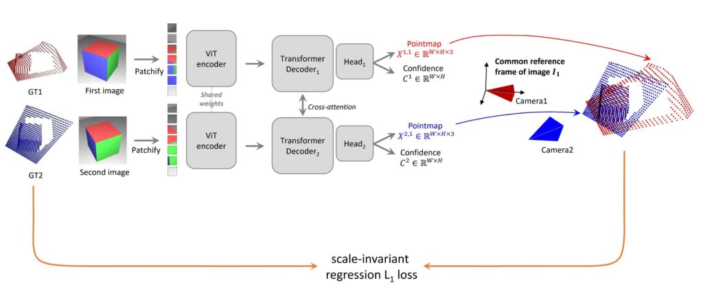
MASt3R extends DUSt3R with an additional descriptor head ( $\text{Head}_{\text{desc}}$ ) that outputs local features and incorporates, optimization strategies for pairwise feature matching with matching loss achieving robust local image matching. Unlike DUSt3R, which uses scale-invariant regression loss, MASt3R employs a variant of cross entropy loss called InfoNCE loss to establish better pixel correspondences while natively outputting metric point maps.

MASt3R (Multi View Stereo 3D Reconstruction) model Architecture. It has two heads one for 3D Reconstruction and other for image matching. Using Fast NN reciprocal matches are retrieved for reducing the search space. It treats image matching as a 3D task — FIG 4: MASt3R Architecture

Given two images of same scene, MASt3R jointly solves geometrical matching and generates a pairwise feature map whose spatial dimensions is similar to input images (HxWxd), where d is the dimension of descriptor vector.

Similar to DUSt3R, pair of images are encoded using ViT encoders in siamese manner (shared weights). MASt3R leverages off-the-shelf weights of DUSt3R, both trained using a similar CroCo pretraining strategy.

AsymmetricMASt3R(
 (patch_embed): PatchEmbedDust3R(
   (proj): Conv2d(3, 1024, kernel_size=(16, 16), stride=(16, 16))
   (norm): Identity()
 )
 (mask_generator): RandomMask()
 (rope): cuRoPE2D()
 (enc_blocks): ModuleList(
   (0-23): MASt3R is fundamentally limited to process image pairs, and it doesn't scale well for larger scenes. Therefore as a followup work MASt3R-SfM.24 x Block(
     (norm1): LayerNorm((1024,), eps=1e-06, elementwise_affine=True)
     (attn): Attention(
     (mlp): Mlp(
       (fc2): Linear(in_features=4096, out_features=1024, bias=True)
      . . .  )))

Then these encoded latent representations ( $H^1$ and $H^2$ ) are decoded by transformer decoders with two heads. The two decoders exchanges the spatial and geometric features and relationships of the given images to establish correspondences via cross attention.

$H'^{1}, H'^{2} = \text{Decoder}(H^{1}, H^{2})$

(decoder_embed): Linear(in_features=1024, out_features=768, bias=True)

# DECODER 1
 (dec_blocks): ModuleList(
   (0-11): 12 x DecoderBlock(
     (norm1): LayerNorm((768,), eps=1e-06, elementwise_affine=True)
     (attn): Attention(. . .)
     (cross_attn): CrossAttention(. . .)
     (mlp): Mlp(
 . . .
(fc2): Linear(in_features=3072, out_features=768, bias=True)
)

# DECODER 2
 (dec_blocks2): ModuleList(
   (0-11): 12 x DecoderBlock(
     (norm1): LayerNorm((768,), eps=1e-06, elementwise_affine=True)
     (attn): Attention(. . .)
     (cross_attn): CrossAttention(. . .)
     (mlp): Mlp(
 . . .
 (fc2): Linear(in_features=3072, out_features=768, bias=True)
) ))

Geometric head ( $\text{Head}^{\text{3D}}$ ) :

For dense 3D Reconstruction, $\text{Head}^{\text{3D}}$ is to generate points maps and confidence values from a pair of images.

(downstream_head2): Cat_MLP_LocalFeatures_DPT_Pts3d(
   (dpt): DPTOutputAdapter_fix(. . . )
     (head): Sequential(
       (0): Conv2d(256, 128, kernel_size=(3, 3), stride=(1, 1), padding=(1, 1))
        . . .
       (4): Conv2d(128, 4, kernel_size=(1, 1), stride=(1, 1))
     )
    . . . 
   (head_local_features): Mlp(
     (fc1): Linear(in_features=1792, out_features=7168, bias=True)
     (fc2): Linear(in_features=7168, out_features=6400, bias=True)
   . . . 
   )
 )

$X^{1,1}, C_1 = \text{Head}_1^{3D}( [H^{1}, H'^{1} ])$ . . . [ 1 ]

$X^{2,1}, C_2 = \text{Head}_2^{3D}( [H^{2}, H'^{2} ])$ . . . [ 2 ]

Dense 3D Reconstruction loss:

In DUSt3R scale-invariant regression loss,

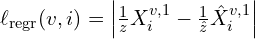
$\ell_{\text{regr}}(v, i) = \left| \frac{1}{z} X_i^{v,1} - \frac{1}{\hat{z}} \hat{X}_i^{v,1} \right|$

where,

$X_i^{v,1}$ is the ground truth 3D point for pixel i in view v
$X_i^{v,1}$ is the predicted 3D point for pixel i in view v
$z$ and $\hat{z}$ is the normalization factor used to make it scale-invariant.

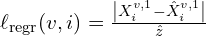
“One of the primary motivation of MASt3R is to solve the relative pose estimation of Map-Free Relocalization benchmark which necessiates the estimates in metric scale”.

MASt3R ignores the normalization factor to make its output metric depth. Therefore the metric regression loss would look as,

$\ell_{\text{regr}}(v, i) = \frac{\left|X_i^{v,1} - \hat{X}_i^{v,1}\right|}{\hat{z}}$

The confidence-aware regression loss to optimize for 3D Reconstruction will be,

$L_{conf} = \sum_{v \in {1,2}}\sum_{i \in V_v} C_v^i \ell_{regr}(v, i) - \alpha \log C_v^i.$

Matching head ( $\text{Head}_{\text{desc}}$ ):

However, MASt3R introduces an additional head ( $\text{Head}_{\text{desc}}$ ) to output dense local features $F^{m, n}$ .

(downstream_head1): Cat_MLP_LocalFeatures_DPT_Pts3d(
   (dpt): DPTOutputAdapter_fix(. . .)
       
   (head_local_features): Mlp(
     (fc1): Linear(in_features=1792, out_features=7168, bias=True)
     (fc2): Linear(in_features=7168, out_features=6400, bias=True)
     . . .
   ) )

Each decoder ( $\text{Head}_{\text{desc}}$ ) outputs two dense local feature maps $D^1, D^2 \in \mathbb{R}^{H \times W \times d},$

$D^1 = \text{Head}^1_{\text{desc}} ( [H^{1}, H'^{1}]), \quad$

$D^2 = \text{Head}^2_{\text{desc}} ( [H^{2}, H'^{2}]), \quad$

Matching loss:

In MASt3R, a pixel i in image 1 and a pixel j in image 2 are considered as true match if they correspond to the same ground truth 3D point. i.e. Each local descriptor in a image matches at max only a single descriptor in the other image. The network is trained to learn such descriptors while penalizing non-matching feature descriptors using InfoNCE loss which is much more effective than a simple 3D regression loss, as used in DUSt3R. This enables MASt3R to learn fine-grained details with sub-pixel level accuracy while being robust to both 3D geometry and scene matching.

The matching loss is essentially a cross-entropy classification loss (InfoNCE),

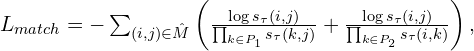
$L_{match} = - \sum_{(i, j) \in \hat{M}} \left( \frac{\log s_\tau (i, j)}{\prod_{k \in P_1} s_\tau (k, j)} + \frac{\log s_\tau (i, j)}{\prod_{k \in P_2} s_\tau (i, k)} \right), \quad$

where, $s_\tau (i, j) = \exp \left( -\tau D_1^\top D_j^2 \right). \quad$

Here,

$\hat{P}_1 = {i \mid (i, j) \in \hat{M}} \quad \text{and} \quad \hat{P}_2 = {j \mid (i, j) \in \hat{M}}$ denotes the subset of pixels considered in each image.
$\tau$ is temperature hyper parameter.

📌 Finally, both regression and matching losses are combined to optimize for the overall training objective of MASt3R,

$L_{total} = L_{conf} + \beta L_{match}$

A simple implementation of these loss functions in PyTorch would be as follows,

# L_conf
def metric_regression_loss(X_pred, X_gt, conf, alpha=0.1):
    """
    Computes the confidence-aware metric regression loss.
    
    Args:
        X_pred (torch.Tensor): Predicted 3D points (B, N, 3)
        X_gt (torch.Tensor): Ground truth 3D points (B, N, 3)
        conf (torch.Tensor): Confidence values (B, N)
        alpha (float): Regularization weight for confidence

    Returns:
        torch.Tensor: Loss value
    """
    norm_factor = X_gt[..., -1].unsqueeze(-1)  # Extracting z as normalization factor
    regr_loss = torch.abs(X_pred - X_gt) / norm_factor
    loss = (conf * regr_loss).sum() - alpha * torch.log(conf).sum()
    return loss

# L_match
def matching_loss(D1, D2, matches, tau=0.07):
    """
    Computes the InfoNCE loss for dense feature matching.

    Args:
        D1 (torch.Tensor): Local descriptors from image 1 (B, H*W, d)
        D2 (torch.Tensor): Local descriptors from image 2 (B, H*W, d)
        matches (torch.Tensor): Binary mask of matching pixels (B, H*W, H*W)
        tau (float): Temperature hyperparameter

    Returns:
        torch.Tensor: Matching loss
    """
    similarity = torch.exp(-tau * torch.bmm(D1, D2.transpose(1, 2)))  # Compute similarity
    pos_pairs = matches * similarity  # Mask out non-matching pairs
    neg_pairs = (1 - matches) * similarity  # Mask out positive pairs

    loss = -torch.log(pos_pairs.sum(dim=-1) / (pos_pairs.sum(dim=-1) + neg_pairs.sum(dim=-1))).mean()
    return loss

Optimization Strategies:

One may wonder when already have 3D point maps, why we need descriptors additionally for matching? As discussed earlier about Route 1 and Route 2, pointmaps can give coarse alignment by directly matching 3D points to 2D pixel positions however they are not accurate. Even small errors in 3D can mean a pixels offseted by centimeters. However MASt3R is specifically trained with an feature matching objective which uses an optimization scheme to refine dense feature maps for coarse to fine matching especially for high resolution images.

Unlike DUSt3R’s Global alignment strategy, MASt3R primarily uses two efficient optimization strategies, which are,

Fast Reciprocal Matching
Coarse to Fine Matching

Fast Recriprocal Matching (FRM)

Reciprocal matching system ensures that if point A in image1 matches point B in image2, then the reverse should also hold true. By this, spurious matches caused by noise, occlusions and perspective distortions are filtered out. However, Naive reciprocal matching techniques is often slow, computationally expensive. To address this inefficiency, MASt3R employs Fast Reciprocal Nearest Neighbor Matching (FRM) which accelerates the matching process by retaining only the most relevant matches.

Difference in matching density - Dense Reciprocal Matching vs Fast Reciprocal Matching with k=3000. FRM converges unformly — FIG 5: Difference in matching density – **Dense Reciprocal Matching** vs Fast Reciprocal Matching with k=3000
FRM converges uniformly

To establish correspondences between the dense feature maps, $D^1$ and $D^2$ FRM begins by sampling an initial sparse set of pixels $U_0$ from first Image $I_1$ .

For each pixel in $U_0$ , the nearest neighbor (NN) in the second image $I_1$ is identified, which forms the set $V_1$ .
To retain only true matches, each pixel in $V_1$ is mapped back to $I_1$ by computing its NN in reverse fashion resulting a corresponding set $U_1$ .
If $U_1$ matches $U_0$ the match is considered reciprocal and they form a cycle.

$U_0 \text{ (Initial set)} \xrightarrow{\text{Find NN in } I_2} V_1 \text{ (Mapped pixels in } I_2)$

$V_1 \xrightarrow{\text{Find NN in } I_1} U_1 \text{ (Mapped pixels back in } I_1 )$

: Illustration of the iterative FRM algorithm. Starting from 5 pixels in 𝐼
1 at 𝑡 = 0, the FRM connects
them to their Nearest Neighbors (NN) in 𝐼
2
, and maps them back to their NN in 𝐼
1
. If they go back to their starting
point (top pink), a cycle (reciprocal match) is detected and returned. Otherwise (bottom) the algorithm continues
iterating until a cycle is detected for all starting samples, or until the maximal number of iterations is reached.
We show in orange the starting points of a convergence basin, i.e. nodes of a sub-graph for which the algorithm
will converge towards the same cycle. For clarity, all edges of G were not drawn. — FIG 6: Detecting cycles iteratively using FRM Algorithm

$M = { (i, j) \mid j = \text{NN}_2(D^1_i) \text{ and } i = \text{NN}_1(D^2_j) }, \quad$

$\text{with } \text{NN}_A (D^B_j) = \mathop{\text{arg min}}_i | D^A_i - D^B_j |$

This iterative process continues up until a stable number of reciprocal pairs are identified and remaining ones are filtered out. This method significantly reduces the search space, making the matching process 64x faster and efficient compared to naive brute force reciprocal search. For FRM, MASt3R pipeline internally uses Faiss library to store correspondences.

Fast reciprocal matching. Left: Illustration of the fast matching process, starting from an initial subset
of pixels 𝑈
0 and propagating it iteratively using 𝑁𝑁 search. Searching for cycles (blue arrows) detect reciprocal
correspondences and allows to accelerate the subsequent steps, by removing points that converged. Center:
Average number of remaining points in 𝑈
𝑡 at iteration 𝑡 = 1 . . . 6. After only 5 iterations, nearly all points have
already converged to a reciprocal match. Right: Performance-versus-time trade-off on the Map-free dataset.
Performance actually improves, along with matching speed, when performing moderate levels of subsampling. — FIg 7: Searching for cycles (blue arrows) detect reciprocal
correspondences and allows to accelerate the subsequent steps

Coarse to Fine Pairwise Matching Scheme

To get this level of accurate correspondences, working with high-res images should be ideal choice. However, ViT’ ‘s has doesn’t generalize well in handling large resolutions. To mitigate this MASt3R uses the clever approach of coarse to fine matching scheme.

Initial Coarse-Scale Matching: The process begins by performing matching on downscaled versions of the input images to obtain initial rough set of coarse correspondences denoted by ${M^0_k}$ .

Window Based Matching ( $w_n$ ): Then to refine these coarse correspondences, MASt3R employs a window-based matching technique on full-resolution images. Multiple local windows undergoes feature matching independently. Then fine correspondences obtained from these window pairs are then mapped back to the original image coordinates and merged.

This multi-scale approach enables MASt3R to achieve precise pixel-level feature matching at the same time balances computationally effiency without losing accuracy due to downscaling.

$D^{w1}, D^{w2} = \text{MASt3R}(I_1^{w1}, I_2^{w2}) \quad$

$M_{w1,w2}^k = \text{fastreciprocalNN}(D^{w1}, D^{w2})$

Training and hyperparams Configurations in MASt3R

MASt3R was trained with a diverse mix of 650K image pairs, sampled equally from 14 datasets including Mapfree, Waymo, VirtualKitti and others. By leveraging the strong 3D priors of DUSt3R, MASt3R enhances existing matching capabilities by using DUSt3R’s pre-trained weights for further training over 35 epochs. Similar to DUSt3R, it is designed to handle varying image ratios at inference by training with different input resolution; however, the largest dimension cropped and resized to 512. The output dimension of feature matching head is d = 24 and the confidence loss weight is set to α = 0.2 while the matching loss weight to β=1 to balance speed and accuracy.

The following table quickly summaries the hyperparameters used during MASt3R training,

Hyper-parameters	fine-tuning
Optimizer	AdamW
Base learning rate	$1e^{-4}$
Weight decay	0.05
Adam $\beta$	(0.9, 0.95)
Pairs per Epoch	650k
Batch size	64
Epochs	35
Warmup Epochs	7
Learning rate schedulers	Cosine decay
Input resolutions	512×384, 512×336, 512×288, 512×256, 512×160
Image Augmentations	Random crop, color jittter
Initialization	DUSt3R

Benchmark Results

MASt3R has demonstrated exceptional performance across multiple benchmarks like DTU MVS, Aachen Day-Night, VirtualKitti, RealEstate10k, CO3D-v2, and other datasets.

MASt3R tops the Map-free visual localization leaderboard which is one the challenging dataset as it the model has to infer spatial information purely from inputs — FIG 8: MASt3R Tops Map-free Localization Benchmark

Notably, in the most challenging Map-Free Localization Benchmark, MASt3R achieved a Virtual Correspondence Reprojection Error (VCRE) Area under Curve (AUC) that is 30% higher than the previous methods, effectively handling extreme viewpoint differences upto 180 degrees-scenarios that can be sometimes ambiguous to humans. This remarkable performance is primarily attributed to MASt3R and DUSt3R’s 3D scene understanding and image matching techniques.

Some of the challenging scenarios where MASt3R works like charm even where there aren't much shared features between images making it the SOTA model on Map-free Visual Localization Dataset — FIG 9: MASt3R performance on Hard Cases

Download Code To easily follow along this tutorial, please download code by clicking on the button below. It's FREE!

Click here to download the source code to this post

Code Walkthrough of MASt3R Image Matching

To set up locally, follow along the instructions outlined in the README of MASt3R Repository. After cloning download the model under checkpoints folder,

mkdir -p checkpoints/
wget https://download.europe.naverlabs.com/ComputerVision/MASt3R/MASt3R_ViTLarge_BaseDecoder_512_catmlpdpt_metric.pth -P checkpoints/

For Dense 3D Reconstruction, you can directly run the gradio demo script provided.

!python3 demo.py --model_name MASt3R_ViTLarge_BaseDecoder_512_catmlpdpt_metric

Next, let’s breakdown the “image matching” code that was provided,

Import utilties

The necessary modules are import from mast3r package and along with standard libraries for visualization.

from mast3r.model import AsymmetricMASt3R
from mast3r.fast_nn import fast_reciprocal_NNs

import mast3r.utils.path_to_dust3r
from dust3r.inference import inference
from dust3r.utils.image import load_images

# visualize a few matches
import numpy as np
import torch
import torchvision.transforms.functional
from matplotlib import pyplot as pl

Load Model and Forward Pass

The model is initialized with pre-trained weights and the load images function preprocesses the pair of images by resizing them to supported size of 512 pixels while maintaining the image ratio.

def main():
    device = 'cuda'
    schedule = 'cosine'
    lr = 0.01
    niter = 300

    model_name = "naver/MASt3R_ViTLarge_BaseDecoder_512_catmlpdpt_metric"
    # you can put the path to a local checkpoint in model_name if needed
    model = AsymmetricMASt3R.from_pretrained(model_name).to(device)
    images = load_images(['dust3r/croco/assets/Chateau1.png', 'dust3r/croco/assets/Chateau2.png'], size=512)
    output = inference([tuple(images)], model, device, batch_size=1, verbose=False)

Fast Reciprocal Matching (FRM)

The inference function computes the dense local descriptors (desc) for both images using MASt3R. Followed by this FRM optimization strategy is employed to identify reciprocal nearest neighbors finding accurate correspondences.

 def main():
   . . .
   # at this stage, you have the raw mast3r predictions
    view1, pred1 = output['view1'], output['pred1']
    view2, pred2 = output['view2'], output['pred2']

    desc1, desc2 = pred1['desc'].squeeze(0).detach(), pred2['desc'].squeeze(0).detach()

    # find 2D-2D matches between the two images
    matches_im0, matches_im1 = fast_reciprocal_NNs(desc1, desc2, subsample_or_initxy1=8,
                                                   device=device, dist='dot', block_size=2**13)

Finding True matches

To avoid spurious matches along the edges, we can filter them as they are often unreliable due to occlusion or partial visibility. Therefore a fixed range is chosen and only valid matches in both the images are retained.

 def main() :
   . . .
    # ignore small border around the edge
    H0, W0 = view1['true_shape'][0]
    valid_matches_im0 = (matches_im0[:, 0] >= 3) & (matches_im0[:, 0] < int(W0) - 3) & (
        matches_im0[:, 1] >= 3) & (matches_im0[:, 1] < int(H0) - 3)

    H1, W1 = view2['true_shape'][0]
    valid_matches_im1 = (matches_im1[:, 0] >= 3) & (matches_im1[:, 0] < int(W1) - 3) & (
        matches_im1[:, 1] >= 3) & (matches_im1[:, 1] < int(H1) - 3)

    valid_matches = valid_matches_im0 & valid_matches_im1
    matches_im0, matches_im1 = matches_im0[valid_matches], matches_im1[valid_matches]

Finally, using matplotlib we will visualize the matches between images.

def main():
   . . .
   # Visualization Utility
    n_viz = 20
    num_matches = matches_im0.shape[0]
    match_idx_to_viz = np.round(np.linspace(0, num_matches - 1, n_viz)).astype(int)
    viz_matches_im0, viz_matches_im1 = matches_im0[match_idx_to_viz], matches_im1[match_idx_to_viz]

    image_mean = torch.as_tensor([0.5, 0.5, 0.5], device='cpu').reshape(1, 3, 1, 1)
    image_std = torch.as_tensor([0.5, 0.5, 0.5], device='cpu').reshape(1, 3, 1, 1)

    viz_imgs = []
    for i, view in enumerate([view1, view2]):
        rgb_tensor = view['img'] * image_std + image_mean
        viz_imgs.append(rgb_tensor.squeeze(0).permute(1, 2, 0).cpu().numpy())

    H0, W0, H1, W1 = *viz_imgs[0].shape[:2], *viz_imgs[1].shape[:2]
    img0 = np.pad(viz_imgs[0], ((0, max(H1 - H0, 0)), (0, 0), (0, 0)), 'constant', constant_values=0)
    img1 = np.pad(viz_imgs[1], ((0, max(H0 - H1, 0)), (0, 0), (0, 0)), 'constant', constant_values=0)
    img = np.concatenate((img0, img1), axis=1)
    pl.figure()
    pl.imshow(img)
    cmap = pl.get_cmap('jet')
    for i in range(n_viz):
        (x0, y0), (x1, y1) = viz_matches_im0[i].T, viz_matches_im1[i].T
        pl.plot([x0, x1 + W0], [y0, y1], '-+', color=cmap(i / (n_viz - 1)), scalex=False, scaley=False)
    pl.show(block=True)  

if __name__ == "__main__":
   main()

Image Matching using MASt3R – One Anchor Image (Reference) vs All

MASt3R vs DUSt3R Matching

Gentle Intro to Traditional SfM Approaches

Structure from Motion (SfM) is a photogrammetry technique that aims to reconstruct a 3D geometry of a scene from a set of 2D images. It is a long standing problem in computer vision encompassing classical computer vision techniques like feature-based methods to modern deep learning techniques.

Structure-from-Motion (SfM) Pipeline having feature extraction, feature matching, estimating camera poses, bundle adjustment to generate 3D Reconstructions — FIG 11: Structure-from-Motion (SfM) Pipeline : [ Source ]

Traditional SfM pipelines such as COLMAP, operate by taking a sequence of images, detecting features points and descriptors images and matching these features across different views. RANSAC is then used to filter out bad matches while maximizing inliers. Using triangulation, camera poses are estimated and iteratively refined using Bundle Adjustment (BA) with an objective to minimize reprojection errors.

Triangulation in SfM where two pixel triangulates to a common 3D point — FIG 12: Triangulation in SfM : [Source ]

Limitations of Traditional SfM:

Traditional SfM methods require the camera intrinsics to be known beforehand limiting their applicability in scenarios where camera parameters are unknown or missing.
These methods typically consider only a handful of keypoints to obtain sparse point clouds discarding the global geometric context of the scene.
They are often time consuming and complex, involving multiple intermediate stages potentially introducing noise.
They don’t handle scenes with low texture or repetitive patters well.
Bundle adjustment, a key step in refining 3D points is computationally intensive especially for larger scenes.
They require highly overlapping image sequences and camera motion for accurate reconstruction.

Although DUSt3R provides a good estimate with just a single forward pass eliminating the need for all complex pipelines in traditional SfM, it gives imprecise global SfM reconstruction. Similarly MASt3R while specifically trained for matching image pairs and it doesn’t scale well for larger scenes.

MASt3R-SfM overcomes these challenges by augmenting the strong image matching capabilities of MASt3R enabling it to handle larger scenes like 1000 images. MASt3R-SfM can be a drop in replacement for typical COLMAP-SfM in Gaussian Splatting. It gets rid of Bundle Adjustment which is computationally expensive in traditional SfM.

Understanding MASt3R-SfM

MASt3R-SfM is a fully integrated SfM pipeline that can handle completely unconstrained collections of images from single image to larger scale scenes. It is simple, scalable and fast, for estimating the 3D geometry of a scene reducing the overall computationally complexity from quadratic to nearly linear.

MASt3R-SfM demonstrates strong performance in challenging conditions such as images with no overlap and zero camera motion sequence. For example, observe the below image,

MASt3R-SfM: Reconstruction from six views sharing same optical center i.e. principal point — FIG 13: Reconstruction from six views sharing same optical center i.e. principal point

Working of MASt3R-SfM Pipeline

In SfM, while extracting shared features by processing all image pairs is infeasible, especially at a scale of around 1000 images. To improve effieciency, only the most relevant image pairs are retrieved using MASt3R encoder. This entire pipeline follows a training free approach, leveraging an off-the-shelf MASt3R’s checkpoint for fast image retrieval due to its great geometric and matching priors.

— STEP 1: Sparse Scene Graph Construction —
Given a large collection of images with unknown camera poses a connectivity graph (also called co-visibility graph) is constructed, where:

Nodes represents image pairs
Edges represent mutual feature correspondences

and all the images must be linked together into a single component.

Therefore a fixed set of anchor images are chosen $N_a$ where remaining images (non-anchor) are linked to their closest keyframe among these 20 keyframes using k-nearest neighbors , forming a graph structure (Typically $N_a$ = 20 and k = 10 ).

Mathematically this graph representation can be formulated as:

$G = (\mathcal{V}, \mathcal{E})$

where:

$\mathcal{V}$ is the set of vertices, where each vertex $I \in \mathcal{V}$ represents an image.
$\mathcal{E}$ is the set of edges, where each edge:
$e = (n, m) \in \mathcal{E}$
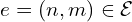
represents an undirected connection between two likely-overlapping images $I_n$ and $I_m$ .

To retrieve the right subset of image pairs, local image features (descriptors) are extracted using MASt3R encoder;

$h(I_n, I_m) \rightarrow s, \text{ where } s \in [0, 1]$

Here, ASMK similarity computed between image representations with a co-visibility score that quanitifies their shared content. A score close to 1 indicates very close similarity with high overlap whereas 0 represents opposite view with no overlap. This ASMK retrieval method is fast and scalable, removing redundancy.

— STEP 2: Local reconstruction —
For each image pair represented by an edge 𝑒 = (𝑛, 𝑚) ∈ E, in the scene graph, the MASt3R decoder computes:

point maps ( $X_{n,m}$ )
sparse pixel matches $M_{n,m}$ representing 2D-3D mappings.

By averaging across image pairs, consistent depth and pose estimates are obtained. For 3D-to-2D projection, the pinhole projective camera model is used (though other camera types can be adapted).

Mathematically,

$M_{n,m} = \{y_{n}^{c} \leftrightarrow y_{m}^{c}\}_{c=1}^{|M_{n,m}|}$

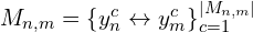
where:

$y_{n}^{c}, y_{m}^{c} \in \mathbb{N}^2$ denote a pair of matching pixel coordinates in images $I_n$ and $I_m$ , respectively.
$|M_{n,m}|$ represents the total number of correspondences.

— STEP 3 — Each local pointmap is aligned to a common world coordinate system in 3D space optimizing using gradient descent based 3D matching loss.

— STEP 4– : To further refine the alignment, the 2D pixel reprojection error is minimised, to ensure better consistency in reconstructed scene and camera poses.

Download Code To easily follow along this tutorial, please download code by clicking on the button below. It's FREE!

Click here to download the source code to this post

Code Walkthrough of MASt3R-SfM Pipeline

MASt3R-SfM is maintained as a separate branch within the MASt3R Repository. You can switch to mast3r-sfm branch for this task. Clone mast3r_sfm branch independently and follow similar instructions to mast3r README.

Make sure to initialize the submodules like CroCo, DUSt3R recursively.

# Open terminal ; create a new environment 
# To only clone the mast3r_sfm branch 
git clone --b mast3r_sfm https://github.com/naver/mast3r.git

cd mast3r
git submodule update --init --recursive

To use MASt3R checkpoint for image retrieval download both the models and place them under the same checkpoints directory.

mkdir -p checkpoints/
wget https://download.europe.naverlabs.com/ComputerVision/MASt3R/MASt3R_ViTLarge_BaseDecoder_512_catmlpdpt_metric_retrieval_trainingfree.pth -P checkpoints/
wget 
#ensure both are in same checkpoint
https://download.europe.naverlabs.com/ComputerVision/MASt3R/MASt3R_ViTLarge_BaseDecoder_512_catmlpdpt_metric_retrieval_codebook.pkl -P checkpoints/

python3 demo.py --model_name MASt3R_ViTLarge_BaseDecoder_512_catmlpdpt_metric 
--retrieval_model checkpoints/MASt3R_ViTLarge_BaseDecoder_512_catmlpdpt_metric_retrieval_trainingfree.pth

Occupies around 11.2 GB for 200 view images, while initial stages ~5GB taking 9 minutes to complete overalll process.

[2025-03-23 16:17:56] init focals = [338.87302 338.87302]
[2025-03-23 16:17:58] >> final loss = 0.0008373452583327889

[2025-03-23 16:18:00] Final focals = [357.24686 357.33545]

python3 demo.py --model_name MASt3R_ViTLarge_BaseDecoder_512_catmlpdpt_metric 
--retrieval_model mast3r/checkpoints/MASt3R_ViTLarge_BaseDecoder_512_catmlpdpt_metric_retrieval_codebook.pkl

Retrieval model

Similar to DUSt3R, MASt3R also has scene graph optimization strategy approaches, such as one-ref, swin or log-win, retrieval. For MASt3R-SfM we will use scene graph strategy of “retrieval: connect views based on similarity” which will fetch the top_k reference images. The codebook.pkl file contains a set of visual descriptors used for image representations to facilitate the matching process.

We have conducted our inference, with the set of configurations shown in the below image,

With retrieval_model the MASt3R-SfM pipeline will look like:

MASt3R →Matching →3D Optimization →2D Refinement →Triangulation →3D Scene.

From the scene graph constructed we can recover:

Focals and Principal Points (intrinsics)
Image Poses (cam2w)
Sparse and Dense 3D Points (pts3d)
Depth Maps (depthmaps)

Feedback: Beginner may feel confused on how to properly setup mast3r_sfm pipeline as the README doesn’t provide clear instructions or differentiation between mast3r main branch.

InstantSplat

After the success of DUSt3R and MASt3R, the team at NVLabs came up with a 3D reconstruction framework InstantSplat which enables to generate accurate 3D representations from as few as 2-3 images. This is a gamechanger replacing the traditional SfM completely and relies on the geometric priors of MASt3R or DUSt3R checkpoints.

To set up locally you can follow the README of official repository “NVlabs/InstantSplat”. However we ran into few issues like the GPU was not recognised and the bash scripts/run_infer.sh wasn’t generating outputs. After further digging we found, jonstephens85 gradio implementation was to the point and simple [ Link ]. We recommend using this for smoother setup.

Then run,

!python instantsplat_gradio.py

The gradio demo expects an input path of the directory containing all images, output directory path and n_views. Modify the following line in the code to allow any arbitrary number of your choice.

# instantsplat_gradio.py 
n_views = gr.Dropdown(choices=[3, 6, 12], value=3, label="Number of Views")
 #     (to)
n_views = gr.TextBox(label="Total images") # len(images)

The pipeline occupies around 11.8GB VRAM for 19 images on a RTX 3080.

Tanks/family – InstantSplat with 19 view

MVImgNet/car- Instant Splat with 19 view

Bungalow – Instant Splat with 19 view

Individuals and enterprises looking to integrate DUSt3R in your workflow and projects, should note that it is licensed under non-commercial (CC BY-NC-SA 4.0) whereas InstantSplat is under Apache 2.0 License.

Key Takeaways

DUSt3R and MASt3R have excellent 3D scene understanding and performs in the wild zero shot. From the predicted 3D geometry focal length can be recovered making these models as a standalone and go to methods for 3D scene reconstruction and pose estimation.
Their success lies in firmly rooting image matching and finding correspondences as 3D in nature.

MASt3R predicts 3D correspondences, even in regions where there aren’t much camera motion or for neatly opposing view of the scene.

MASt3R SfM can do 3D Reconstruction of image collections as large as of 1000 images in one forward pass

Despite MASt3R-SfM pipeline, leverages sparse matches, it can output dense correspondence for every pixel as it uses inverse reprojection error ( $\pi^{-1}$ ) in its training objective. As a result it can provide extremely precise reconstruction for creating highly realistic 3D scenes instantly for larger scenes.

Conclusion

DUSt3R and MASt3R have emerged as promising foundational models for 3D Reconstruction and matching showing excellent generalization across scenes. Inspired from these research advancements, the community have developed several followup works such as VGGT, Fast3R, Spann3R, MonST3R etc.

In this article, we have taken an indepth look at MASt3R, MASt3R-SfM and InstantSplat for larger scenes. In our upcoming article in this 3D Reconstruction series, we will cover MASt3R-SLAM an interesting project that has been gaining traction online.

Hope you find this read interesting. Do let us know your feedback via our social handles.

MASt3R and MASt3R-SfM Explanation: Image Matching and 3D Reconstruction Results

MASt3R: Grounding Image Matching in 3D

What is Image matching?

MASt3R Model Architecture

Geometric head ( $\text{Head}^{\text{3D}}$ ) :

Dense 3D Reconstruction loss:

Matching head ( $\text{Head}_{\text{desc}}$ ):

Matching loss:

Optimization Strategies:

Fast Recriprocal Matching (FRM)

Coarse to Fine Pairwise Matching Scheme

Training and hyperparams Configurations in MASt3R

Benchmark Results

Code Walkthrough of MASt3R Image Matching

MASt3R vs DUSt3R Matching

Gentle Intro to Traditional SfM Approaches

Limitations of Traditional SfM:

Understanding MASt3R-SfM

Working of MASt3R-SfM Pipeline

Code Walkthrough of MASt3R-SfM Pipeline

Retrieval model

InstantSplat

Key Takeaways

Conclusion

References

Get Started with OpenCV

Subscribe to receive the download link, receive updates, and be notified of bug fixes

Which email should I send you the download link?

MASt3R: Grounding Image Matching in 3D

What is Image matching?

MASt3R Model Architecture

Geometric head () :

Dense 3D Reconstruction loss:

Matching head ():

Matching loss:

Optimization Strategies:

Fast Recriprocal Matching (FRM)

Coarse to Fine Pairwise Matching Scheme

Training and hyperparams Configurations in MASt3R

Benchmark Results

Code Walkthrough of MASt3R Image Matching

MASt3R vs DUSt3R Matching

Gentle Intro to Traditional SfM Approaches

Limitations of Traditional SfM:

Understanding MASt3R-SfM

Working of MASt3R-SfM Pipeline

Code Walkthrough of MASt3R-SfM Pipeline

Retrieval model

InstantSplat

Key Takeaways

Conclusion

References

Subscribe & Download Code

Get Started with OpenCV

Subscribe to receive the download link, receive updates, and be notified of bug fixes

Which email should I send you the download link?

Geometric head ( $\text{Head}^{\text{3D}}$ ) :

Matching head ( $\text{Head}_{\text{desc}}$ ):