Iterative Closest Point (ICP) is a widely used classical computer vision algorithm for 2D or 3D point cloud registration. As the name suggests it iteratively improves and minimizes the spatial discrepancies or sum of square errors between two point clouds. The is achieved by estimating an optimal rigid transformation ![]() (Rotation and Translation) matrices that better aligns the “source” or reference point set to a “target” point set in a common coordinate system. It finds huge applications in Medical Imaging, 3D, SLAM, Autonomous Vehicles and Robotics.
(Rotation and Translation) matrices that better aligns the “source” or reference point set to a “target” point set in a common coordinate system. It finds huge applications in Medical Imaging, 3D, SLAM, Autonomous Vehicles and Robotics.
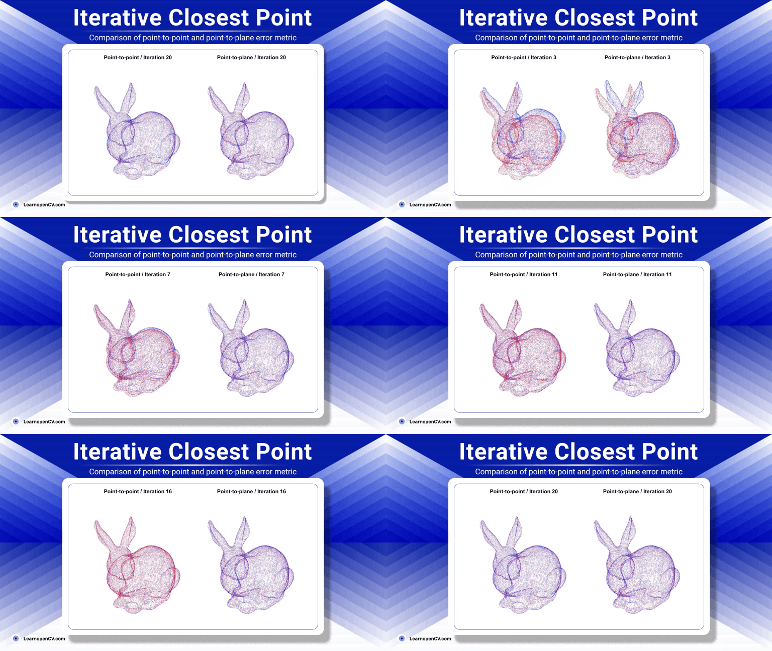
ICP was first formalized by Besl and McKay and the concept dates back to 1992. Since then ICP has evolved quite a lot with numerous variants with notable improvements mainly targeted at robust correspondence matching, weighted error metrics, and acceleration structures for nearest-neighbor search.
In this article, we will provide an overview of ICP, its pipeline, variants and real world use cases along with a demo example using Open3D.
If you’re someone just getting started with 3D computer vision, our series of articles will guide through the fundamentals of 3D Vision and Reconstruction.
- 3D Reconstruction with Gaussian Splatting and NeRF
- Stereo and Monocular Depth Estimation
- Understanding Camera calibration and Geometry.
- Monocular Visual SLAM
- DUSt3R: Dense 3D Reconstruction
- MASt3R and MASt3R-SfM
- VGGT: VGGT: Visual Geometry Grounded Transformer
- MASt3R-SLAM: Real-Time Dense SLAM
- What is point cloud registration?
- Pipeline of Iterative Closest Point (ICP)
- Practical Considerations for ICP’s Performance
- Common ICP Variants
- Code Walkthrough of ICP
- Real-world use cases of ICP
- Conclusion
- References
What is point cloud registration?
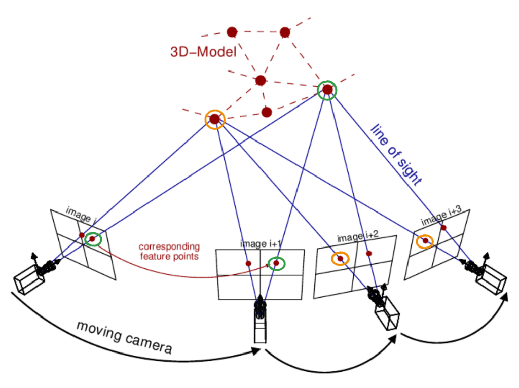
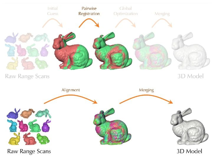
A point cloud is essentially a set of vertices in a 3D coordinate system represented by P = {p_1, p_2, …, p_N}, where each ![]() . To construct a 3D Reconstruction of an object (eg: of a statue), we start by capturing the scene at multiple angles. The source of point set can be either LiDAR , RGB or stereo cameras where each scan produces a separate point cloud.
. To construct a 3D Reconstruction of an object (eg: of a statue), we start by capturing the scene at multiple angles. The source of point set can be either LiDAR , RGB or stereo cameras where each scan produces a separate point cloud.
The challenge lies in combining features of multiple scans of an object captured from different views or at different time intervals into a single coherent structure without gaps, deformation or outliers. To create a intact geometry out of it, we need to meticulously stitch them together. The process of finding the precise rotation and translation that aligns the source point cloud to target point cloud in a common coordinate system is called registration.
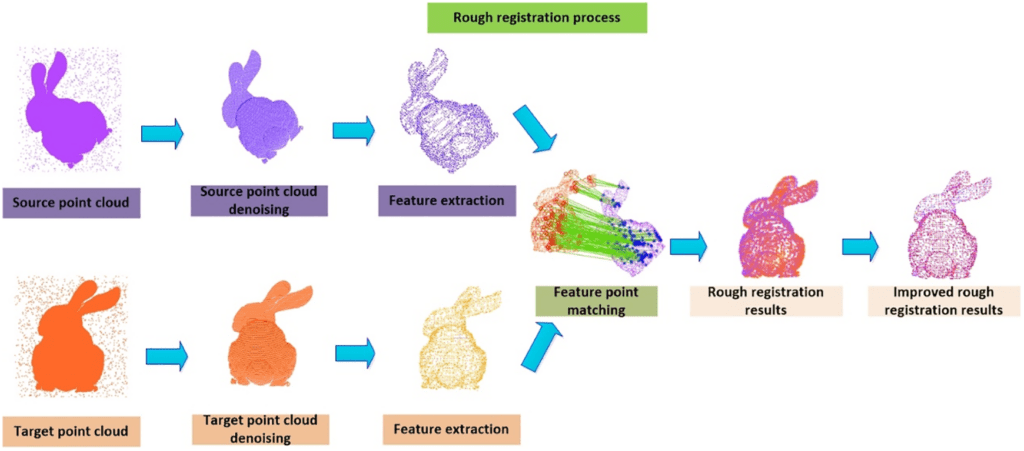
It starts with an initial guess for the transformation and is refined step-by-step until a convergence criterion is met. The intuitive idea behind ICP is if we knew the correspondence points between the source and target cloud, finding the best transformation is straightforward mathematically. On the otherhand if we knew the correct transformation, finding corresponding points is pretty simple and they will perfectly align. But we know neither, therefore ICP alternates between estimating correspondences and estimating transformation based on initial correspondences. If two point cloud came from same source, we aren’t concerned about scaling.

Despite its conceptual simplicity, ICP’s effectiveness hinges on factors such as initialization quality, choice of error metric and strategies for outlier rejection.
Pipeline of Iterative Closest Point (ICP)
Standard ICP algorithm has the following steps:
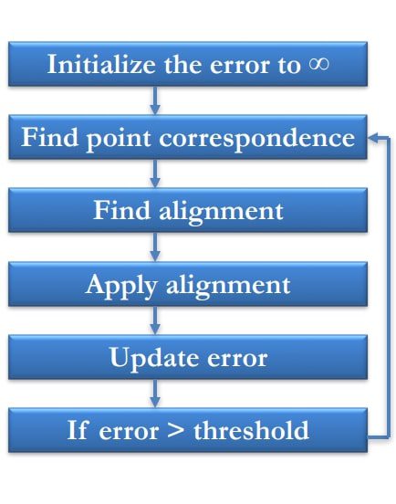
Step 1: Initialization
ICP doesn’t start from scratch; it begins with an initial estimate of the transformation ![]() that roughly aligns the source cloud
that roughly aligns the source cloud ![]() to the target cloud
to the target cloud ![]() .
.
![]()
Here ![]() represents the source cloud after applying the initial transformation. The quality of initial guess is crucial; a poor initialization can lead ICP to converge to an incorrect algorithm (a local minima) or fail to converge at all.
represents the source cloud after applying the initial transformation. The quality of initial guess is crucial; a poor initialization can lead ICP to converge to an incorrect algorithm (a local minima) or fail to converge at all.
The initial guess might come from:
- Sensor priors (GPS/IMU data on a mobile scanner)
- Manual placement by the user,
- Matching distinctive features between clouds.
- The output of global registration algorithm (which provides a rough alignment). We initialize counter
 .
.
Step 2: Finding Correspondences
For each point ![]() in the current iteration’s transformed source cloud
in the current iteration’s transformed source cloud ![]() , find the closest point
, find the closest point ![]() in the target point cloud
in the target point cloud ![]() . “Closest” is typically defined by the Euclidean distance. This steps establishes a set of relevant corresponding pairs
. “Closest” is typically defined by the Euclidean distance. This steps establishes a set of relevant corresponding pairs ![]() .
.
However finding matching pairs for every point in the cloud is computationally expensive. To overcome this bottleneck, the most common approach is to build a k-d tree on static target cloud ![]() . A k-d tree partitions the 3D space recursively, allowing for efficient nearest neighbor search. This results in significant speeding the process as it reduces the search space by finding nearest neighbors of query point from
. A k-d tree partitions the 3D space recursively, allowing for efficient nearest neighbor search. This results in significant speeding the process as it reduces the search space by finding nearest neighbors of query point from ![]() ,
,
Step 3: Estimating Transformation
Given the set of matching pairs ![]() found in the previous step, the algorithm computes the rigid transformation (
found in the previous step, the algorithm computes the rigid transformation (![]() ) that best align these pairs. By minimizing sum of squared Euclidean distance between the transformed source points and their corresponding target points.
) that best align these pairs. By minimizing sum of squared Euclidean distance between the transformed source points and their corresponding target points.
![]()
The optimization problem has a closed-form solution. A common and robust method to find the optimal rotation ![]() and translation
and translation ![]() involves using Singular Value Decomposition (SVD). First the centroids (mean position) of the corresponding source points (
involves using Singular Value Decomposition (SVD). First the centroids (mean position) of the corresponding source points (![]() ) are calculated. Then, centroid points are computed:
) are calculated. Then, centroid points are computed: ![]() and
and ![]() .
.
A cross-variance matrix is formed as sum of the outer products of these centered corresponding pairs,
![]()
Applying SVD to this matrix ![]() yields three matrices,
yields three matrices,
![]() .
.
Here,
 and
and  are orthogonal matrices representing rotations/reflections
  is a diagonal matrix containing single values.
The optimal rotation matrix ![]() is then calculated as
is then calculated as ![]() . A special check is often needed: if the determinant of
. A special check is often needed: if the determinant of ![]() is -1 (indicating a reflection rather than a proper rotation), the sign of the last column of
is -1 (indicating a reflection rather than a proper rotation), the sign of the last column of ![]() is typically flipped before recalculating
is typically flipped before recalculating ![]() to ensure it’s a valid rotation matrix. Once the optimal rotation
to ensure it’s a valid rotation matrix. Once the optimal rotation ![]() is found, the optimal translation
is found, the optimal translation ![]() is easily computed using the centroids
is easily computed using the centroids
![]()
Step 4: Applying the Transformation
Then update the source point cloud by applying newly computed transformation ![]() . Often, the transformation is accumulated relative to the original source cloud
. Often, the transformation is accumulated relative to the original source cloud ![]() rather than iteratively transforming the points themselves, to avoid potential drift.
rather than iteratively transforming the points themselves, to avoid potential drift.
![]()
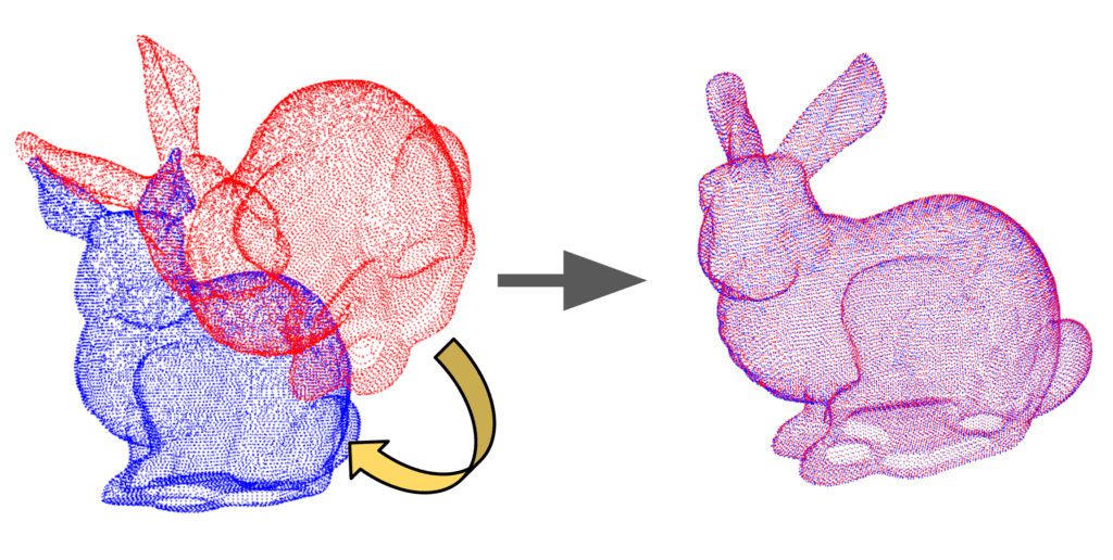
Step 5: Checking Convergence
The algorithm checks if a termination condition has been met. Common convergence criteria include:
- The relative change in the mean squared error (calculated in Step 3) between iterations falls below a predefined threshold.
- The relative change in the transformation parameters (R and t) between iterations falls below a threshold.
- A maximum number of iterations has been reached.
If the convergence criteria are met, the algorithm terminates and outputs the final transformation (![]() ). Otherwise, increment
). Otherwise, increment ![]() (i.e.,
(i.e., ![]() ) and return to Step 2. Find the best possible matches between two clouds and find the correspondences. Given this try to optimize the translation and rotation
) and return to Step 2. Find the best possible matches between two clouds and find the correspondences. Given this try to optimize the translation and rotation
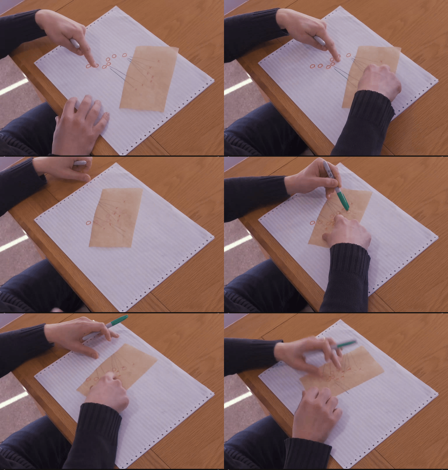
Iterative Closest Point ICP Computerphile
Iterative Closest Point ICP Computerphile
Practical Considerations for ICP’s Performance
While the pipeline seems straightforward, several factors heavily influence ICP’s real-world effectiveness:
- Initialization and Local Minima: As mentioned, ICP is a local optimization algorithm. It finds the best alignment within the nearest neighbors of the initial guess. If initial guess is poor, ICP can easily get stuck in local minima – an alignment that looks locally optimal might be globally correct. Ensuring a reasonable starting position, often through rough initial alignment or global registration techniques, is crucial. Therefore the initial pose is chosen in such a way that it assumes that at start there is sufficient overlap between the source and target.
- Outlier Sensitivity: The standard least-square error metric is highly sensitive to outliers-incorrect correspondences caused by noise, non-overlapping regions or dynamic objects. A few bad matches can significantly skew the transformation estimate. Strategies to mitigate this include:
- Distance thresholding: Rejecting pairs whose distance exceeds a certain value.
- Percentage Rejection: Discarding a fixed percentage of pairs with largest errors.
- Robust Error Metrics: Using metrics less sensitive to outliers, like the sum of absolute differences (L1 norm) or more advanced robust functions (eg., Huber loss).
- Random Sample Consensus (RANSAC): Iteratively selecting minimal subset of pairs to estimate transformations and finding the one supported by the most inliers.
- Computation Cost: Even with k-d trees, processing large point clouds can be time-consuming. Techniques to manage this include:
- Point Sampling: Using only a subset of points from the source cloud (e.g., random sampling, uniform sampling, or selecting points in high-curvature areas).
- Multi-Resolution Approaches: Performing ICP initially on downsampled versions of the point clouds for a coarse alignment, then gradually increasing the resolution for refinement.
Common ICP Variants
The basic ICP algorithm (often called Point-to-Point ICP) has inspired many variants aimed at improving convergence speed and accuracy:
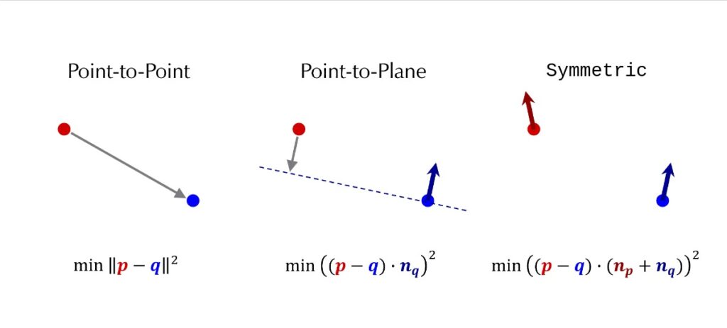
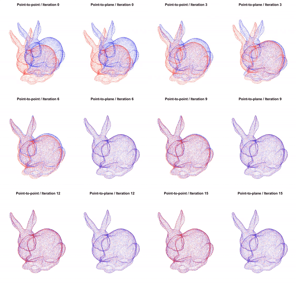
- Point-to-Point ICP : This is the classic or standard ICP which establishes correspondences by finding the closest point in the target cloud for each point in the source cloud. The objective is to minimize the sum of squared euclidean distances directly between these corresponding points. While straightforward its convergence can be slower in some scenarios, and it relies purely on point proximity.
![]()
- Point-to-Plane ICP : Instead of minimizing the direct distance between corresponding points, this popular variant minimizes the distance from each source point to the tangent plane at its corresponding target point. This requires estimating surface normals for the target cloud (and sometimes the source cloud). The error metric changes to reflect this point-to-plane distance. This approach often leverages the underlying surface geometry more effectively, leading to faster convergence and higher accuracy, especially for scenes with flat or structured surfaces.
![]()
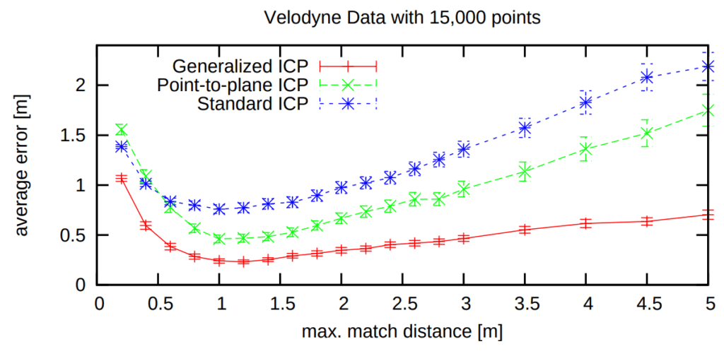
- Plane-to-Plane (Generalized ICP-G-ICP): This methods extends the idea further by modeling uncertainity and local planarity (using covariance matrices) in both the source and target clouds. It effectively minimizes a distance between locally planar patches, often resulting in greater robustness to noise and varying point densities compared to point-to-point or point-to-plane methods.
- Symmetric ICP : In standard ICP, correspondences are usually found from the source to the target cloud only. Symmetric ICP considers correspondences in both directions (source-to-target and target-to-source) simultaneously during the optimization process. This can sometimes improve stability and prevent the alignment from drifting in one direction.
Code Walkthrough of ICP
First, we will visualize ICP from Open3D demo examples. Then, we will implement a very simple version of ICP in python to understand its underlying mechanism.
Using Open3D
!pip install open3d
Import Dependencies
import numpy as np
import matplotlib.pyplot as plt
import open3d as o3d
import copy
Import Dataset
We will load two example point clouds (source and target) from the Open3D ICP demo dataset, each representing a 3D scan of a room captured at different view.
# Read source and target PCD
demo_pcds = o3d.data.DemoICPPointClouds()
source = o3d.io.read_point_cloud(demo_pcds.paths[0]) # PointCloud with 191397 points.
#source.dimension( )  -> 3
target = o3d.io.read_point_cloud(demo_pcds.paths[1]) # PointCloud with 137833 points.
#target.dimension( )  -> 3
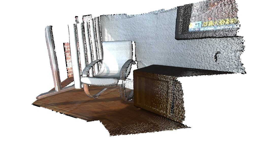
Visualize Input Before Registration
o3d.visualization.draw_plotly([source],
                                  zoom=0.455,
                                  front=[-0.4999, -0.1659, -0.8499],
                                  lookat=[2.1813, 2.0619, 2.0999],
                                  up=[0.1204, -0.9852,Q 0.1215])

o3d.visualization.draw_plotly([target],
                                  zoom=0.455,
                                  front=[-0.4999, -0.1659, -0.8499],
                                  lookat=[2.1813, 2.0619, 2.0999],
                                  up=[0.1204, -0.9852, 0.1215])
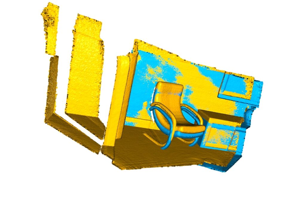
Initial Registration Obtained from Global Registration
The function below visualizes a target point cloud and a source point cloud transformed with an rough initial alignment transformation. The target point cloud and the source point cloud are painted with cyan and yellow colors respectively. The more and tighter the two point clouds overlap with each other, the better the alignment result.
def draw_registration_result(source, target, transformation):
      source_temp = copy.deepcopy(source)
      target_temp = copy.deepcopy(target)
      source_temp.paint_uniform_color([1, 0.0706, 0])
      target_temp.paint_uniform_color([0, 0.651, 0.929])
      source_temp.transform(transformation)
      o3d.visualization.draw_plotly([source_temp, target_temp])


# *** Initial Transformation ***
trans_init = np.asarray([[0.862, 0.011, -0.507, 0.5],
                         [-0.139, 0.967, -0.215, 0.7],
                         [0.487, 0.255, 0.835, -1.4], [0.0, 0.0, 0.0, 1.0]])

draw_registration_result(source, target, trans_init)
The function evaluate_registration calculates two main metrics:
fitness, which measures the overlapping area (# of inlier correspondences / # of points in source). The higher the better.inlier_rmse, which measures the RMSE of all inlier correspondences. The lower the better.
By default, registration_icp runs until convergence or reaches a maximum number of iterations (30 by default). It can be changed to allow more computation time and to improve the results further.
threshold = 0.02
print("Initial Alignment")
evaluation = o3d.pipelines.registration.evaluate_registration(
                       source, target, threshold, trans_init)
print(evaluation)

"""Initial alignment
RegistrationResult with fitness=2.740900e-02, inlier_rmse=1.259521e-02, and correspondence_set size of 5246
Access transformation to get result."""
Registration through use of ICP
- Point-to-Point
- Point-to-Plane
The class TransformationEstimationPointToPoint provides functions to compute the residuals and Jacobian matrices of the point-to-point ICP objective. The function `registration_icp` takes it as a parameter and runs point-to-point ICP to obtain the results.
Point-to-Point
# ******* Point-to-Point *********
threshold = 0.02
print("Apply point-to-point ICP")
reg_p2p = o2d.pipelines.registration.registration_icp(
                   source, target, threshold, trans_init,
                   o3d.pipelines.registration.TransformationEstimationPointToPoint())
print(reg_p2p)
print("Transformation is:")
print(reg_p2p.transformation)
draw_registration_result(source, target, reg_p2p.transformation)

"""
Apply point-to-point ICP
RegistrationResult with fitness=3.132755e-02, inlier_rmse=1.168464e-02, and correspondence_set size of 5996
Access transformation to get result.
Transformation is:
[[ 0.86481662  0.0378514  -0.50084398  0.42597758]
 [-0.15157681  0.97072361 -0.18799414  0.66535821]
 [ 0.47817432  0.23769297  0.84517011 -1.35537445]
 [ 0.          0.          0.          1.        ]]
"""
The fitness score increases from 0.174723 to 0.372450. The inlier_rmse reduces from 0.011771 to 0.007760.
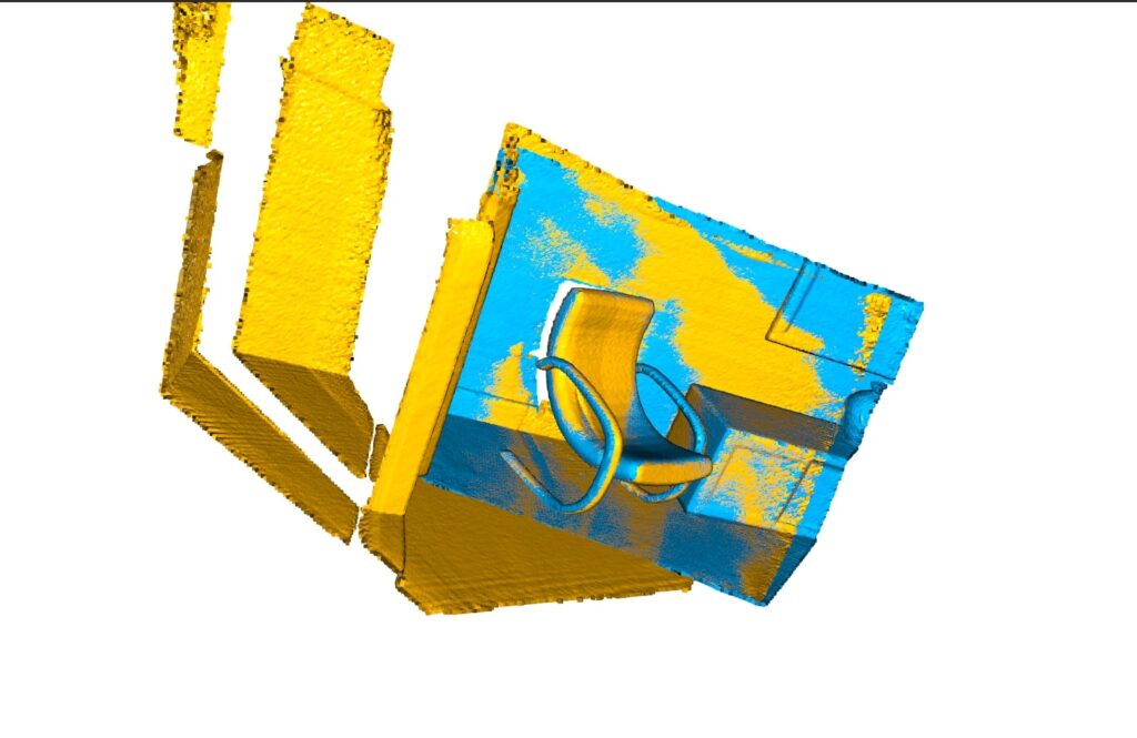
Point-to-Plane
The point-to-plane ICP algorithm uses point normals. In this tutorial, we load normals from files. If normals are not given, they can be computed with Vertex normal estimation. `registration_icp` is called with a different parameter TransformationEstimationPointToPlane. Internally, this class implements functions to compute the residuals and Jacobian matrices of the point-to-plane ICP objective.
threshold=0.02
print("Apply point-to-point ICP")
reg_p2p = o3d.pipelines.registration.registration_icp(
    source, target, threshold, trans_init,
    o3d.pipelines.registration.TransformationEstimationPointToPoint())
print(reg_p2p)
print("Transformation is:")
print(reg_p2p.transformation)
draw_registration_result(source, target, reg_p2p.transformation)
The point-to-plane ICP reaches tight alignment within 30 iterations (a fitness score of 0.620972 and an inlier_rmse score of 0.006581).
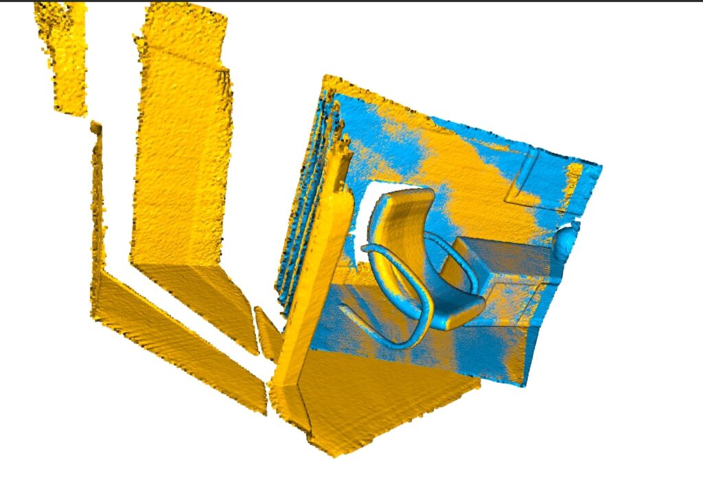
Simple Implementation
Aligning two sinusoidal point clouds that are originally identical, but is subjected to a homogeneous transformation. ICP algorithm progressively brings the two point clouds into alignment by minimizing their distance.
Import dependencies
import numpy as np
from sklearn.neighbors import NearestNeighbors
import matplotlib.pyplot as plt
import matplotlib.animation as animation
The best_fit_transform function implements a least-squares best-fit transformation algorithm that maps matching points (correspondences) between two two point clouds (A and B). It calculates the rotation matrix, translation vector and the homogeneous transformation matrix required to transform A onto B.
Steps:
- Check that A and B have same shape
- Calculate the centroids of A and B and translates the points into their centroids
- Calculate the rotation matrix using SVD. If the determinant of the rotation matrix is negative, reflect the last row of Vt.
- Calculate translation using the transformed centroids and the rotation matrix
- Construct homogeneous transformation matrix using the rotation matrix and translation vector.
def best_fit_transform(A, B):
    """
    Calculates the best-fit transform that maps points A onto points B.
    Input:
        A: Nxm numpy array of source points
        B: Nxm numpy array of destination points
    Output:
        T: (m+1)x(m+1) homogeneous transformation matrix
    """
    assert A.shape == B.shape
    m = A.shape[1]
    centroid_A = np.mean(A, axis=0)
    centroid_B = np.mean(B, axis=0)
    AA = A - centroid_A
    BB = B - centroid_B
    H = np.dot(AA.T, BB)
    U, S, Vt = np.linalg.svd(H)
    R = np.dot(Vt.T, U.T)
    if np.linalg.det(R) < 0:
       Vt[m-1,:] *= -1
       R = np.dot(Vt.T, U.T)
    t = centroid_B.reshape(-1,1) - np.dot(R, centroid_A.reshape(-1,1))
    T = np.eye(m+1)
    T[:m, :m] = R
    T[:m, -1] = t.ravel()
    return T
Next to find the nearest neighbors between the destination and source point clouds. The function nearest_neighbor` takes in two inputs src and dst and returns the euclidean distances and indices of the nearest neighbor in dst for each point in src using kd-tree.
def nearest_neighbor(src, dst):
    '''
    Find the nearest (Euclidean) neighbor in dst for each point in src
    Input:
        src: Nxm array of points
        dst: Nxm array of points
    Output:
        distances: Euclidean distances of the nearest neighbor
        indices: dst indices of the nearest neighbor
    '''
    # Ensure shapes are compatible for KNN, although they don't strictly need to be identical N
    assert src.shape[1] == dst.shape[1]
    neigh = NearestNeighbors(n_neighbors=1)
    neigh.fit(dst)
    distances, indices = neigh.kneighbors(src, return_distance=True)
    return distances.ravel(), indices.ravel()
The following function implements the ICP algorithm iteratively updates the transformation between updated A and B. The iterations repeats until the difference between the mean error of the closest point distances between the current and previous iterations is less than a tolerance value specified or until the maximum number of iterations is reached. The output is the final homogeneous transformation matrix T_final that maps A onto B to reach convergence.
To visualize the convergence through all the steps we will also need to store the intermediate steps.
# --- Modified ICP function to store history ---
def iterative_closest_point_visual(A, B, max_iterations=20, tolerance=0.001):
    '''
    The Iterative Closest Point method: finds best-fit transform that maps points A on to points B.
    Stores intermediate results for visualization.
    Input:
        A: Nxm numpy array of source points
        B: Nxm numpy array of destination points
        max_iterations: exit algorithm after max_iterations
        tolerance: convergence criteria
    Output:
        T_final: final homogeneous transformation that maps A on to B
        intermediate_A: List containing A transformed at each iteration (N x m arrays)
        intermediate_errors: List containing the mean error at each iteration
        i: number of iterations to converge
    '''

    # Check dimensions
    # Allow N to differ, but dimensions (m) must match
    assert A.shape[1] == B.shape[1]

    # get number of dimensions
    m = A.shape[1]

    # --- Store History ---
    intermediate_A = [np.copy(A)] # Store initial state
    intermediate_errors = []
    # --- Store History ---

    # make points homogeneous, copy them to maintain the originals
    # Use np.copy() for src to allow modification without affecting original A
    src_h = np.ones((m+1, A.shape[0]))
    src_h[:m, :] = np.copy(A.T)

    # Target points (B) remain fixed, use non-homogeneous for KNN
    dst = np.copy(B) # Non-homogeneous target points for KNN

    prev_error = float('inf') # Initialize with infinity
    T_cumulative = np.identity(m+1) # To accumulate transformations correctly

    for i in range(max_iterations):
        # Current source points (non-homogeneous)
        current_src = src_h[:m, :].T

        # find the nearest neighbors between the current source and destination points
        distances, indices = nearest_neighbor(current_src, dst)

        # compute the transformation between the current source and nearest destination points
        # Use the subset of B (dst) corresponding to the nearest neighbors found
        T_step = best_fit_transform(current_src, dst[indices, :])

        # update the current source points *in homogeneous coordinates*
        src_h = np.dot(T_step, src_h)

        # --- Store History ---
        intermediate_A.append(src_h[:m, :].T) # Store transformed A for this iteration
        # --- Store History ---

        # check error (stop if error is less than specified tolerance)
        mean_error = np.mean(distances)
        intermediate_errors.append(mean_error) # Store error for this iteration

        # Use absolute difference check for convergence
        if np.abs(prev_error - mean_error) < tolerance:
            print(f"Converged at iteration {i+1} with error difference {np.abs(prev_error - mean_error)}")
            break

        prev_error = mean_error

        # Accumulate transformation
        T_cumulative = np.dot(T_step, T_cumulative)


    # Calculate the *final* transformation from the *original* A to the *final* src position
    # This accounts for the accumulated transform
    T_final = best_fit_transform(A, src_h[:m, :].T)

    # If loop finished due to max_iterations without converging based on tolerance
    if i == max_iterations - 1:
         print(f"Reached max iterations ({max_iterations})")

    return T_final, intermediate_A, intermediate_errors, i + 1 # Return i+1 for actual count
# Define two sets of points A and B (same as your example)
t = np.linspace(0, 2*np.pi, 10)
A = np.column_stack((t, np.sin(t)))

# Define the rotation angle
theta = np.radians(30)
c, s = np.cos(theta), np.sin(theta)
rotation_matrix = np.array(((c, -s), (s, c)))

# Define translation vector
translation_vector = np.array([[2, 0]])

# Apply the transformation and add randomness to get B
np.random.seed(42) # for reproducible randomness
randomness = 0.3 * np.random.rand(10, 2)
B = np.dot(rotation_matrix, A.T).T + translation_vector + randomness

# --- Run ICP and get history ---
max_iter = 20
tolerance = 0.0001 # Lower tolerance for smoother convergence potentially
T_final, history_A, history_error, iters = icp.iterative_closest_point_visual(A, B, max_iterations=max_iter, tolerance=tolerance)

print(f'Converged/Stopped after {iters} iterations.')
print(f'Final Mean Error: {history_error[-1]:.4f}')
print('Final Transformation:')
print(np.round(T_final, 3))
# --- Create Animation ---
fig, ax = plt.subplots()

# Plot target points (static)
ax.scatter(B[:, 0], B[:, 1], color='blue', label='Target B', marker='x')

# Plot initial source points
scatter_A = ax.scatter(history_A[0][:, 0], history_A[0][:, 1], color='red', label='Source A (moving)')
title = ax.set_title(f'Iteration 0, Mean Error: N/A')
ax.legend()
ax.set_xlabel("X")
ax.set_ylabel("Y")
ax.grid(True)
ax.axis('equal') # Important for visualizing rotations correctly

# Determine plot limits based on all points across all iterations
all_points = np.vstack([B] + history_A)
min_vals = np.min(all_points, axis=0)
max_vals = np.max(all_points, axis=0)
range_vals = max_vals - min_vals
margin = 0.1 * range_vals # Add 10% margin
ax.set_xlim(min_vals[0] - margin[0], max_vals[0] + margin[0])
ax.set_ylim(min_vals[1] - margin[1], max_vals[1] + margin[1])

# Animation update function
def update(frame):
    # Update source points position
    scatter_A.set_offsets(history_A[frame])
    # Update title
    error_str = f"{history_error[frame-1]:.4f}" if frame > 0 else "N/A" # Error calculated *after* step
    title.set_text(f'Iteration {frame}, Mean Error: {error_str}')
    # Return the artists that were modified
    return scatter_A, title,

# Create the animation
# Number of frames is number of states stored (initial + iterations)
# Interval is milliseconds between frames (e.g., 500ms = 0.5s)
ani = animation.FuncAnimation(fig, update, frames=len(history_A),
                              interval=500, blit=True, repeat=False)

# Display the final plot (optional, animation already shows it)
plt.figure()
plt.scatter(history_A[-1][:, 0], history_A[-1][:, 1], color='red', label='Final A')
plt.scatter(B[:, 0], B[:, 1], color='blue', label='Target B', marker='x')
plt.legend()
plt.title(f"Final Alignment after {iters} iterations")
plt.xlabel("X")
plt.ylabel("Y")
plt.grid(True)
plt.axis('equal')
plt.show()
Real-world use cases of ICP
- SLAM: In robotics and autonomous driving, ICP is fundamental for scan matching. By aligning consecutive sensor scans (eg, from LiDAR), robots estimate their motion (odometry) and build consistent maps of their environment. Modern state-of-the-art SLAM systems often use sophisticated ICP variants. For eg: KISS-ICP and GenZ-ICP
“good old ICP still stands strong when done right“
- Medical Imaging: Aligning medical scans taken at different modalities or times to track disease propagation, plan surgeries or guide interventions.
- Manufacturing and Quality Control: Comparing 3D scans of manufactured parts against their digital CAD models to detect defects and ensure tolerances are met (metrology).
- Augmented/Virtual Reality (AR/VR): Aligning virtual objects with real-world point cloud data enables realistic integration and interaction within mixed reality environments (hololens) ensuring proper placement and scaling.
Advantages of ICP
- Precise Fine Alignment: Highly effective at refining alignment when given a decent starting point
- Simplicity: The core iterative idea is easy to grasp and implement
- Robust : Enhanced versions (e.g., point-to-plane) handle noise, outliers, and featureless areas better.
Disadvantages of ICP
- Requires good initial guess: Very prone to failing (local minima) if the start alignment is poor. If two point clouds doesn’t have sufficient overlap, then the alignment might fail to converge.
- Computationally expensive: Can be slow, especially for large point clouds
- Sensitive to Outliers/Low Overlap: The standard version struggles significantly with noise, incorrect pairings, and limited overlap.
Conclusion
We discussed indepth about Iterative Closest Point algorithm and understood how the mathematical formulation turns out in python code. While deep learning based methods and sophisticated registration techniques are advantageous for complex scenarios, ICP’s core principle offer a simple and effective approach that sometimes even outperforms state-of-art SLAM algorithms in specific scenarios. This highlights that classical computer vision algorithms are still relevant and fundamental blocks across many applications.
Hope you find this read interesting. Do let us know your feedback via our social handles.
References
- ICP – Computerphile
- Cyrill Stachniss
- ICP Open3D Example Tutorial
- Simple Implementation of ICP
- A Tutorial on Rigid Registration







100K+ Learners
Join Free OpenCV Bootcamp3 Hours of Learning