IoU Loss Functions for Faster & More Accurate Object Detection

Object detection is one of the most important challenges in computer vision. Deep learning-based solutions can solve it very effectively. To solve any problem using deep learning, first, we need to model the problem as an optimization problem and then optimize it using some iterative optimization technique (e.g., gradient descent). The object detection loss function choice is crucial in modeling an object detection problem. Generally, object detection needs two loss functions, one for object classification and the other for bounding box regression. This article will focus on IoU loss functions (GIoU loss, DIoU loss, and CIoU loss). But first, we will gain an intuitive understanding of the loss function for object detection in general.

The article is most beneficial to those:

Who wants to read and understand the paper- Generalized Intersection over Union: A Metric and A Loss for Bounding Box Regression, by H Rezatofighi et al.
Who want insights into the paper – Distance-IoU Loss: Faster and better learning for Bounding Box Regression, by Z Zheng et al.
Who wants a general understanding of the bounding box regression loss function for object detection.

In this article, we will discuss only regression loss for object detection. If you are not already familiar with object detection fundamentals and pipelines, the following article may be helpful:

MSE Loss Function
IoU Loss Functions
GIoU (Generalized IoU) Metric and Loss Function
DIoU (Distance IoU) Loss Function
CIoU (Complete IoU) Loss Function
NMS (Non-Maximum Suppression) using DIoU
IoU, GIoU, DIoU, and CIoU Loss Comparison
DIoU/CIoU Convergence Compare to GIoU
Summary
Further Readings
References

Before going into the IoU-based loss function, let us look at the traditional regression loss function (MSE, MAE, combined) for object detection. Let us understand its pitfalls, thereby concluding that we need a better loss function.

MSE Loss Function

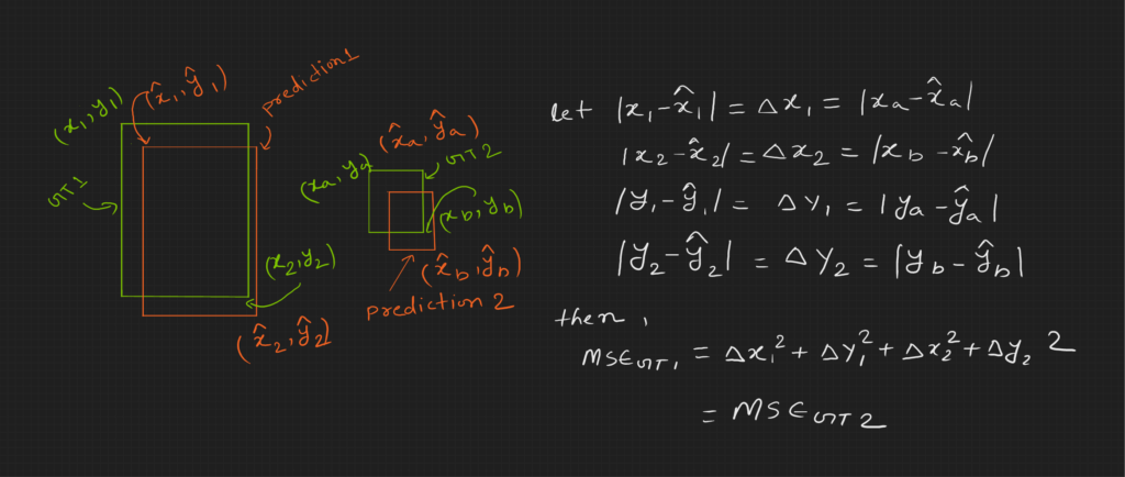
MSE Loss for Object Detection Regression - object detection loss function — <strong>MSE Loss for Object Detection Regression<strong>

In the above image, we can see that the prediction for the larger object is very close to the ground truth, and the prediction for the smaller object seems far from the ground truth. However, the distance of predictions from their ground truth is the same in both cases. This means that the loss and the gradient will be the same. Let’s look at the gradients of MSE and MAE loss functions.

Gradients of MSE and MAE Loss Functions

Let us plot $MAE\text{-vs.-}\Delta{x}$ and $MSE\text{-vs.-}\Delta x$ to understand loss and gradient.

MSE and MAE Loss Function and Its Gradients. — <strong>MSE and MAE Loss Function and Its Gradients<strong>

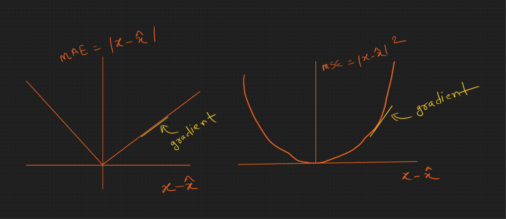
The above plot shows that loss and gradient is the only function of $\Delta x$ . The gradient is fixed for a given $\Delta x$ . So it implies that both predictions will have the same contribution to the weight update of the model. However, intuitively the smaller object prediction should have more contribution. But it is not the case here. It could be a better loss function.

IoU Loss Functions

Why IoU-based loss functions are a better choice compared to MSE or MAE?

The mAP (mean average precision) metric in object detection is evaluated based on IoU (Intersection Over Union). Hence it is better to use the IoU-based loss function to achieve a better mAP.

Problem with Typical IoU Loss Function

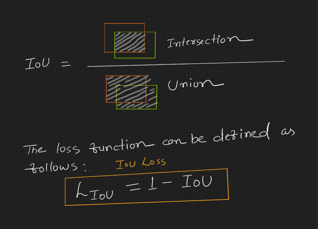
IoU Loss Functions - Object detection loss function — <strong>IoU Loss Function<strong>

The problem with the IoU (above) loss function is that if there are no overlaps between ground truth and prediction, the IoU is zero, and the gradient is also zero – why is the gradient zero?

When IoU is zero, the loss will be 1 (one minus zero), which is constant. Hence with no change in loss, the gradient will be zero.

The gradient is zero in case of no overlap; this is not a good loss function because the initial predictions (during training) will likely be in that situation.

Can we modify the above equation to use it as a proper loss function?

Yes. GIoU (Generalized Intersection over Union) has some modifications to repurpose the above equation as a better loss function.

GIoU (Generalized IoU) Metric and Loss Function

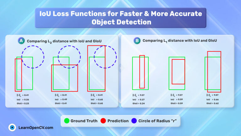
Before going into the GIoU metric/loss, look at the image below.

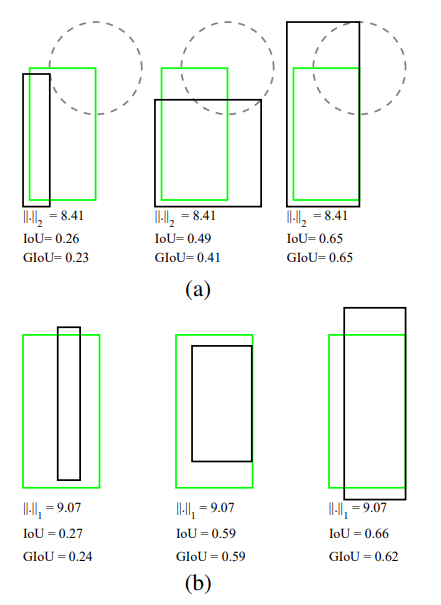
MSE or MAE vs. IoU or GIoU - Object detection loss function — <strong>MSE or MAE vs IoU or GIoU<strong>

In the above image, there are two sets of examples, (a) and (b), with the bounding boxes represented by (a) two corners $(x_1, y_1, x_2, y_2)$ and (b) center and size $(x_c, y_c, w, h)$ . For all three cases in each set, (a) $l_2-norm$ distance, $||.||_2$ , and (b) $l_1-norm$ distance, $||.||_1$ , between the representations of two rectangles are the same value, but their IoU and GIoU values are very different.

It means that in the case of MSE or MAE, the quality of the bounding is not adequately represented by the loss function. This also states that MSE or MAE is not a good loss function for object detection regression.

As discussed earlier, the IoU does not distinguish between close and far predictions if it has no overlap with the ground truth. However, GIoU does that.

The equation for GIoU is:

$GIOU = IoU - \frac{C \backslash (A \cup B)}{C}$

Here, $C$ is the smallest convex object that encloses $A$ and $B$ . However, the authors used the smallest rectangles that enclose both $A$ and $B$ .

Let us see how we can calculate $C$ in the figure below.

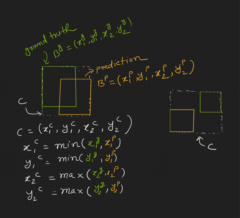
Note that, $0 \leq IoU \leq1$ but $-1 < GIoU < 1$ .

GIoU loss:

$L_{GIoU} = 1 - GIoU = 1 - IoU + \frac{C \backslash (A \cup B)}{C}$

For $IoU=0$ , the loss is not fixed; instead, it depends on how far the prediction and ground truth boxes are. So it is a better loss function compared to IoU. Because even if IoU is zero, it has a gradient to push the bounding box toward the ground truth.

The GIoU loss function is better than IoU and MSE. Here is a comparison table to back it up.

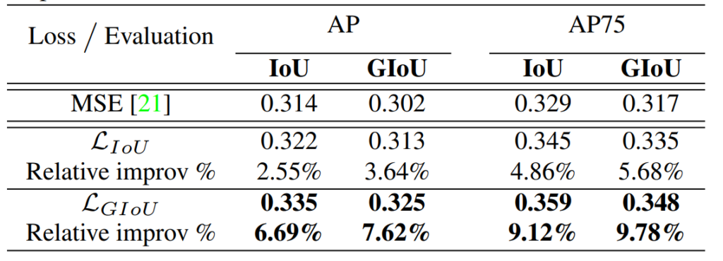
<strong>GIoU Loss is Better than MSE and IoU Loss<strong>

The table is a performance comparison of YOLOv3 trained on the COCO dataset with different loss functions – (i) MSE, YOLOv3 original loss, (ii) IoU loss, and (iii) GIoU loss.

GIoU is a winner with a considerable margin.

DIoU (Distance IoU) Loss Function

Before going into detail about DIoU, look at the figure below.

IoU and GIoU vs. DIoU - object detection loss function — <strong>IoU and GIoU vs DIoU<strong>

In the above figure, the green bounding box is the ground truth, and the red is a prediction.

We can see above that IoU and GIoU are the same for all three. However, DIoU is different. DIoU is the same as IoU and GIoU in the third (left to right), where prediction and ground truth centers are the same (DIoU is the minimum). It means DIoU loss pushes the prediction center to the ground truth center.

DIoU Loss Function

DIoU loss is defined as follows:

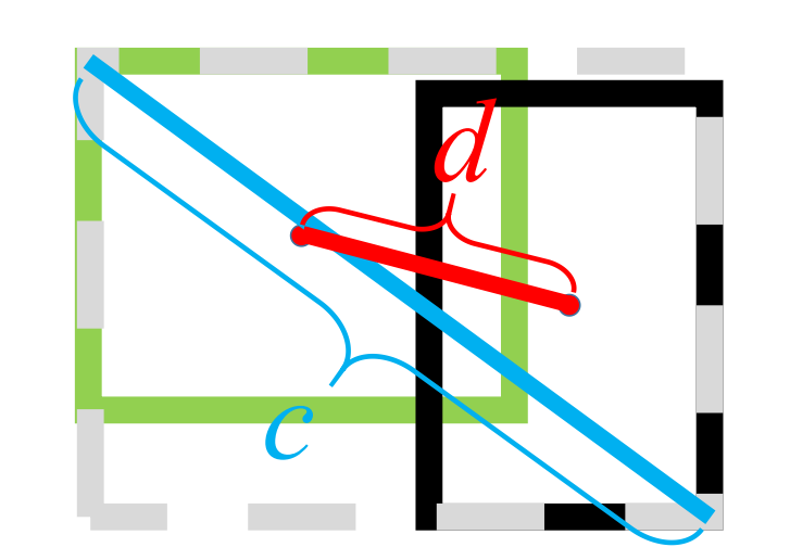
Distance in DIoU - Object detection loss function — <strong>Distance in DIoU<strong>

$L_{DIoU} = 1 - IoU + \frac{d^2}{C^2}$

DIoU Loss Converges Faster Compared to IoU and GIoU Loss

Let us look at the effectiveness of DIoU loss compared to IoU and GIoU loss.

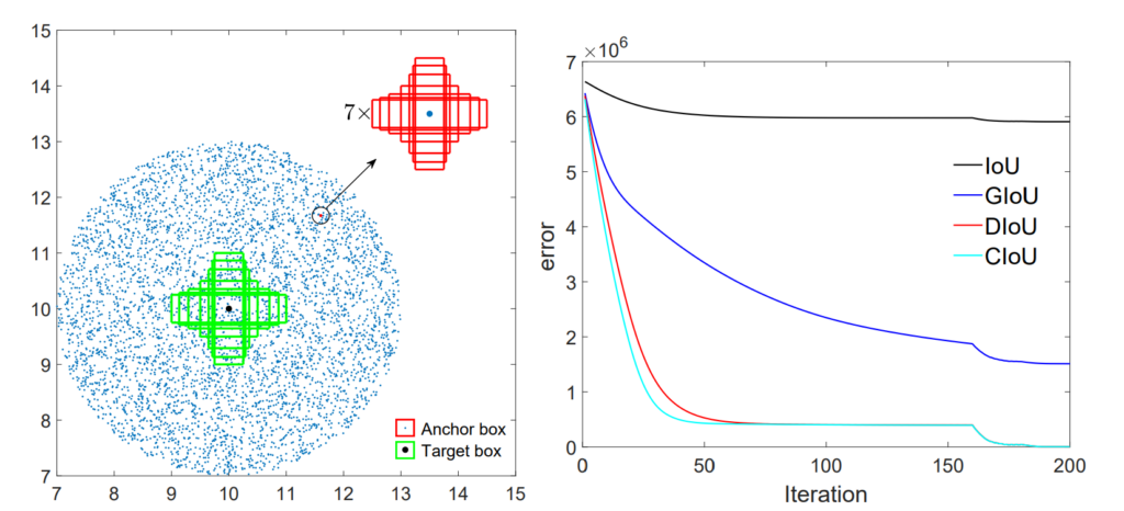
DIoU Simulation Experiment - IoU loss functions - Object detection loss function — <strong>DIoU Simulation Experiment<strong>

Here is a simulation experiment. There are seven targets (green) with fixed areas and seven aspect ratios. There are 5000 points for anchor boxes around the target boxes, as shown in the above image. At each point, there are 49 anchors (seven sizes and seven aspect ratios). Each anchor has seven regression cases for seven targets. So at each anchor point, there are 7 x 7 x 7 regression targets.

IoU, GIoU, DIoU, and CIoU (discussed next) loss functions achieve these regression targets. The loss plot for different IoU loss functions is shown on the right side of the above image. DIoU and CIoU are much better compared to IoU and GIoU. The convergence of DIoU and CIoU is much faster than IoU and GIoU.

DIoU has Lower Losses Compared to IoU and GIoU

Have a look at the image below.

Regression Error at the Final Step at Every Anchor Box Coordinate - IoU loss functions - object detection loss function — <strong>Regression Error at the Final Step at Every Anchor Box Coordinate<strong>

The above plot is a regression error at the final step at every coordinate.

Why are IoU losses high?

For IoU loss, points far from the target’s losses are high. This is expected because distant point prediction may not overlap with the targets that lead to zero IoU; hence no further optimization in the case of IoU loss.

Why are GIoU losses high at the horizontal and vertical orientations?

Loss for GIoU loss function is better than IoU loss function. However, the horizontal and vertical orientation cases will still likely have significant errors. And the reason is in the image below.

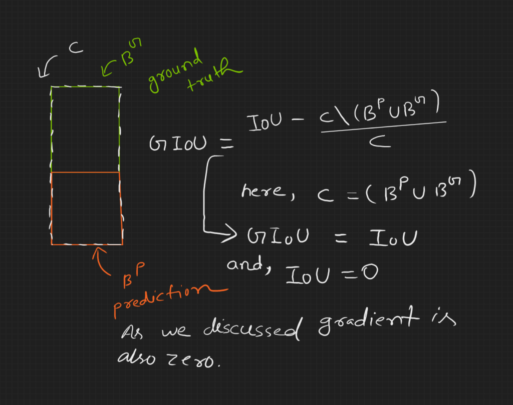
GIoU Fails at Horizontal and Vertical Orientations - IoU loss functions - object detection loss function — GIoU Fails at Horizontal and Vertical Orientations

Loss for DIoU loss function is much better than GIoU loss function. It is because it does not depend on the orientation of the anchor box to ground truth.

CIoU (Complete IoU) Loss Function

This is an extension of DIoU loss. Additionally, which also accommodates deviation of aspect ratio.

The CIoU loss function:

$L_{CIoU} = 1 -IoU + \frac{d^2}{C^2} + \alpha v$

where,

$v = \frac{4}{\pi^2}(arctan\frac{w^{gt}}{h^{gt}} - arctan\frac{w}{h})^2$

$\alpha$ is a trade-off parameter and is defined as:

$\alpha = \frac{v}{(1-IoU) + v}$

$\alpha$ is a function of IoU. The above equation states that the aspect ratio factor is less important in the case of no overlap and more important in the case of more overlap.

NMS (Non-Maximum Suppression) using DIoU

Instead of IoU, DIoU can be used for NMS. DIoU-NMS can be formally defined as:

$s_i = \begin{cases} s_i, & IoU - \frac{d^2}{C^2} < \epsilon,\\ 0, & \text{otherwise} \end{cases}$

If the two predicted bounding box overlap sufficiently, but their center is far, most probably, the bounding boxes belong to different objects.

IoU, GIoU, DIoU, and CIoU Loss Comparison

A quantitative comparison of YOLOv3 (Redmon and Farhadi) trained using $L_{IoU}$ (baseline), $L_{GIoU}$ , $L_{DIoU}$ , and $L_{CIoU}$ . $(D)$ denotes-using $DIoU-NMS$ . PASCAL VOC 2007 test set is used to report the result.

IoU vs. GIoU vs. DIoU vs. CIoU - Object detection loss function — <strong>IoU vs GIoU vs DIoU vs CIoU <strong>

DIoU/CIoU Convergence Compare to GIoU

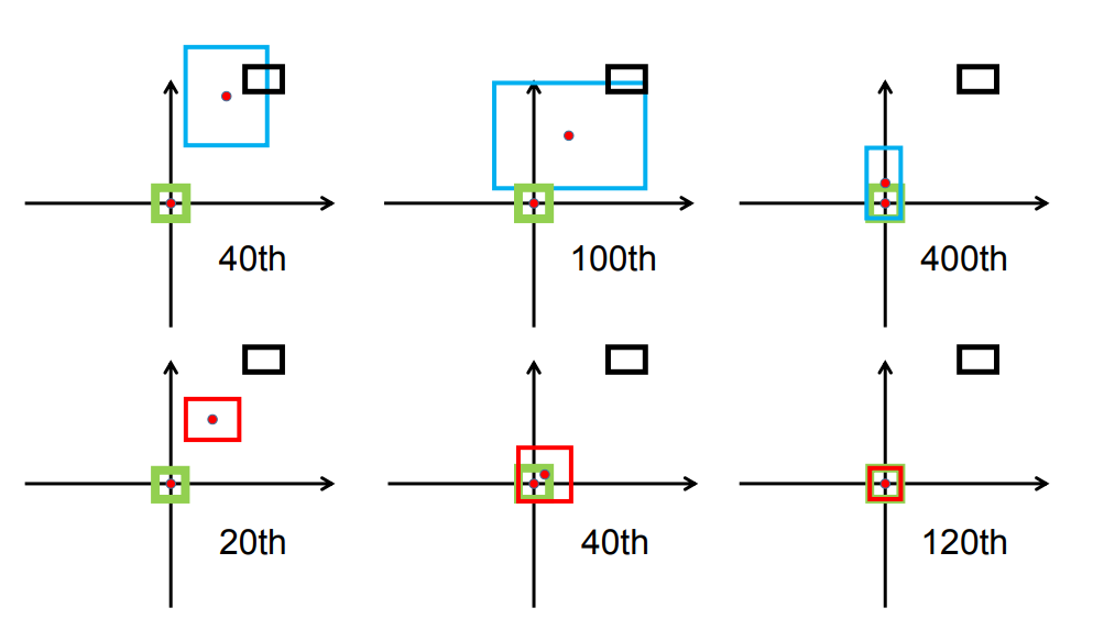
DIoU/CIoU vs. GIoU Convergence - IoU loss functions - object detection loss functions — <strong>DIoUCIoU vs GIoU Convergence<strong>

The first row is for GIoU, and the second is for DIoU. Green boxes are targets. Black boxes are anchors. Blue and red boxes are predictions for GIoU and DIoU loss, respectively.

We can see that convergence to target is faster for DIoU loss than GIoU loss.

Summary

CIoU loss function is better than GIoU and DIoU.
Nowadays, the CIoU loss function is commonly used for object detection regression.
For NMS, using DIoU instead of IoU as the threshold is better.
DIoU and CIoU have much faster convergence compared to GIoU.