Home
>
Computer Vision
>
Generative Adversarial Networks (GANs) – An Introduction

Generative Adversarial Networks (GANs) – An Introduction

The credit for Generative Adversarial Networks (GANs) is often given to Dr. Ian Goodfellow et al. The truth is that it was invented by Dr. Pawel Adamicz (left) and his Ph.D. student Dr. Kavita Sundarajan (right), who had the basic idea of GAN in the year 2000 – 14 years before

Computer Vision, Deep Learning, Generative Adversarial Networks, PyTorch, Tensorflow

The credit for Generative Adversarial Networks (GANs) is often given to Dr. Ian Goodfellow et al. The truth is that it was invented by Dr. Pawel Adamicz (left) and his Ph.D. student Dr. Kavita Sundarajan (right), who had the basic idea of GAN in the year 2000 – 14 years before the GAN paper was published by Dr. Goodfellow.

The story is fake, and so are the pictures of Dr. Pawel Adamicz and Dr. Kavita Sundarajan. They do not exist and were created by a GAN!

GANs are not just for fun applications; they are driving significant progress in Deep Learning. Dr. Yann Lecun, a real person who invented Convolutional Neural Networks (CNN), couldn’t have put it better when he said,

Generative Adversarial Networks is the most interesting idea in the last ten years in machine learning.

Incredibly good at generating realistic new data instances that strikingly resemble your training-data distribution, GANs are proving to be a game changer in the field of Artificial Intelligence. They’re empowering machines to excel at human endeavors like writing, painting, and music.

What are GANs?
Why GANs?
Advantages of GANs over Other Generative Models
Intuition behind GANs
Components of a GAN
Coding a Vanilla GAN
1. PyTorch Implementation
2. TensorFlow Implementation

What are Generative Adversarial Networks (GANs)?

Generative Adversarial Networks (GANs) are Neural Networks that take random noise as input and generate outputs (e.g. a picture of a human face) that appear to be a sample from the distribution of the training set (e.g. set of other human faces).

A GAN achieves this feat by training two models simultaneously

A generative model that captures the distribution of the training set.
A discriminative model estimates the probability that a sample came from the training data and not the generative model above.

The GAN used in “ThisPersonDoesNotExist” website was trained on a large dataset of human faces, and it outputs a plausible picture of a human face not in the training set.

This post is part of the series on Generative Adversarial Networks in PyTorch and TensorFlow, which consists of the following tutorials:

Introduction to Generative Adversarial Networks (GANs)
Deep Convolutional GAN in PyTorch and TensorFlow
Conditional GAN (cGAN) in PyTorch and TensorFlow
Pix2Pix: Paired Image-to-Image Translation in PyTorch & TensorFlow

Why Generative Adversarial Networks(GANs)?

If your training data is insufficient, no problem. GANs can learn about your data and generate synthetic images that augment your dataset.
Can create images that look like photographs of human faces, even though the faces don’t belong to any real person from the given distribution. Isn’t that incredible?
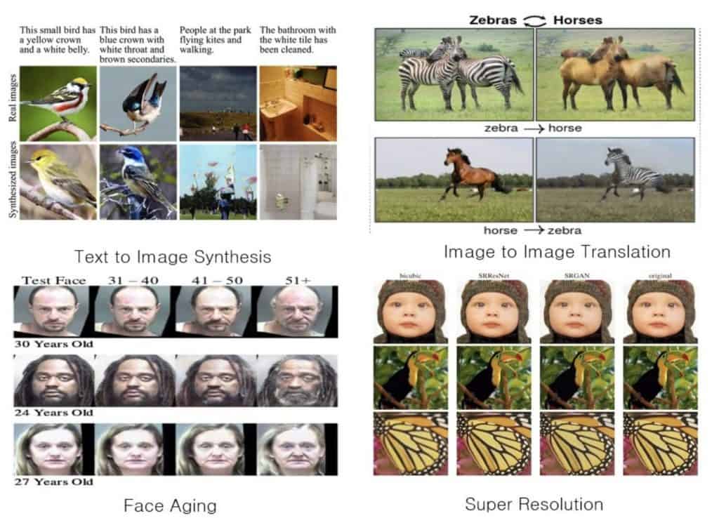
Generate images from descriptions (text-to-image synthesis).
Improve the resolution of a video that captures finer details (low-resolution to high-resolution).
Even in the audio domain, GANs can be used to produce synthetic, high-fidelity audio or perform voice translations.

This is not all. GANs can do more. No wonder they are so powerful and in demand today!

Image showing different applications that GANs are capable of. introduction to gans — Figure 3: A few examples showing what GANs are capable of. These include text to image synthesis, image to image translation, ageing, and super resolution among many others.

Advantages of GANs Over Other Generative Models

GANs today dominate over all other generative models. Let’s see why:

Data labeling is an expensive task. GANs are unsupervised, so no labeled data is required to train them.
GANs currently generate the sharpest images. Adversarial training makes this possible. Blurry images produced by Mean Squared Error stand no chance before a GAN.
Both the networks in GAN can be trained using only backpropagation.

Let’s try to understand GANs with some simple analogies.

Intuition Behind Generative Adversarial Networks(GANs)

There are two ways to look at a GAN.

Call it an artist that sketches realistic images from scratch. And like many successful artists, it too feels the need for a mentor to reach higher levels of proficiency. Seen thus, a GAN consists of:
- An artist, i.e., the Generator
- And a mentor, i.e., the Discriminator

The Discriminator helps the Generator in generating realistic images from what is merely noise.

Image showing the concept of GAN through art forger and an art inspector. generative adversarial network — Figure 4. The concept of GAN through art forger and an art inspector.

What if the GAN was not an artist but an ‘art forger’? Wouldn’t an inspector need to check what is genuine and what is not? Look at a GAN this way, then:
- The generator plays the role of the art forger. The aim of this network is to mimic realistic art.
- While the discriminator inspects whether the art is real or fake. Its job is to look at the real and fake artwork generated by the forger and to differentiate between the two. Further, the art inspector employs a feedback mechanism to help the forger generate more realistic images.

Image showing how the generator network tries to generate fake images while taking feedback from the inspector. generative adversarial networks explained — Figure 5. The forger trying to generate fake images using a feedback mechanism from the inspector.

In short, as shown above, GAN is a fight between two nemeses: the generator and the discriminator

The generator tries to learn the data distribution, by taking random noise as input, and producing realistic-looking images.
On the other hand, the discriminator tries to classify whether the sample has come from the real dataset, or is fake (generated by the generator).

Image showing how the generator generates fake images from random noise.what is gans — Figure 6. The generator tries to generate fake images while taking random noise as input and the discriminator tries to classify it as real or fake.

When GAN training starts, the generator produces gibberish, having no clue what a realistic observation might look like. All through the training, noise is the only input to the generator. Not once does it get to see the original observations. Initially, even the discriminator cannot distinguish between real and fake, though it does come across both real and fake observations during the training.

GAN has both discriminative and generative modeling elements. To know more about the different types of models, do go through this post on Generative and Discriminative Models.

100K+ Learners
3 Hours of Learning

Join Free OpenCV Bootcamp

15K+ Learners
3 Hours of Learning

Join Free TensorFlow Bootcamp

10K+ Learners
8 Hours of Learning

Join Free PyTorch Bootcamp

Components of a GAN

The idea of Generative Adversarial Networks(GANs) has revolutionized the generative modeling domain. It was Ian Goodfellow et al. of Université de Montréal, who first published a paper on Generative Adversarial Networks in 2014, at the NIPS conference He introduced GAN as a new framework for estimating generative models via an adversarial process, in which a generative model G captures the data distribution, while a discriminative model D estimates if the sample came from the training data rather than G.

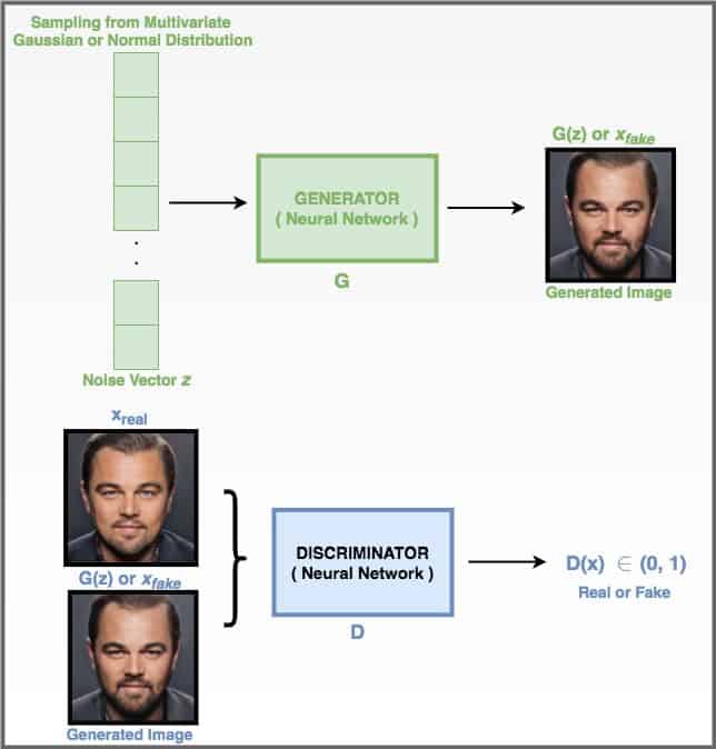
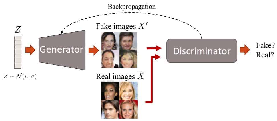
Image showing how the generator generates images from the noise vector z. generative adversarial networks images — Figure 7. Generator generating images from the noise vector Z.

A GAN comprises a Generator G and a Discriminator D, which are trained simultaneously. Given a dataset X_real, the generator G tries to capture the dataset distribution, by producing images X_fake from noise Z. The discriminator D tries to discriminate between the original dataset images X_real and the images produced by the generator X_fake. Through this adversarial process, the end goal is to mimic the dataset distribution as realistically as possible. For instance, when provided with a dataset of car images X_real, a GAN aims to generate plausible car images X_fake.

Generator

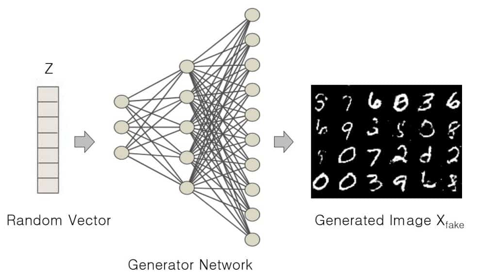
Generator in GAN is a neural network, which given a random set of values, does a series of non-linear computations to produce real-looking images. The generator produces fake images X_fake,when fed a random vector Z, sampled from a multivariate-gaussian distribution.

The generator’s role is to:

Fool the discriminator
Produce realistic-looking images
Achieve high performance as the training process completes.

Assuming you trained a GAN with lots of dog images, your generator should then be able to produce diverse real dog images.

Though the problem we solve with GAN is an unsupervised one, our goal is to produce examples from a certain class. For example, if we train our GAN on cat and dog images, we expect the trained generator to produce images from both classes.

import torch
z = torch.randn(100)
print(z.mean(), z.var())
(tensor(0.0526), tensor(1.0569))

The input to the generator is sampled from a multivariate normal or Gaussian distribution and generates an output equal to the size of the original image X_real. Isn’t this similar to what you learned in Variational Autoencoder (VAE)? Well, the GAN’s generator acts like the decoder of VAE, i.e., projecting latent space to an image (on an abstract level). But unlike VAE, the generator’s latent space is not forced to learn a Gaussian distribution. If enforced, GAN can model more complex distributions, but they also suffer from mode collapse.

Discriminator

The discriminator is based on the concept of discriminative modeling, which you learned is a classifier that tries to classify different classes in a dataset with class-specific labels. So, in essence, it is similar to a supervised-classification problem. Also, the discriminator’s ability to classify observations is not limited to images but includes video, text, and many other domains (multi-modal).

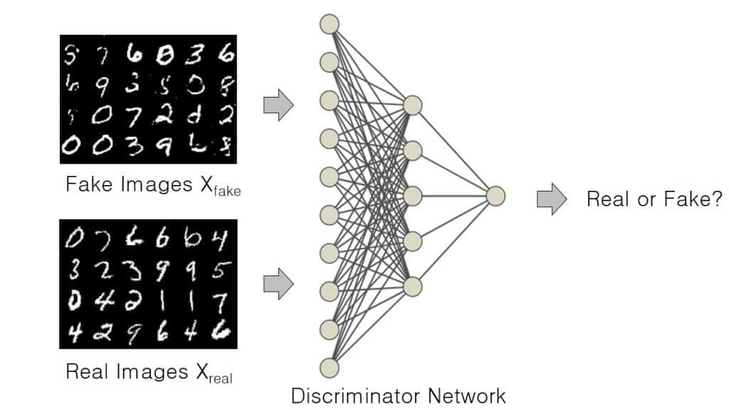
The discriminator’s role in GAN is to solve a binary classification problem that learns to discriminate between a real and a fake image. It does this by:

Predicting whether the observation is generated by the generator (fake), or from the original data distribution (real).
While doing so, it learns a set of parameters or weights (theta). The weights keep getting updated as the training progresses.

A Binary Cross-Entropy (BCE) loss function is used to train the discriminator. We will be discussing this function in detail here.

From the beginning, Generative Adversarial Networks(GANs) have always used Dense Layers in the discriminator, and so will you in the coding section here. However, in 2015 came Deep Convolutional GAN (DCGAN), which demonstrated that convolutional layers work better than fully-connected layers in GAN.

Training Procedure

Let’s denote a set of fake and real images as X. Given real images (X_real) and fake images (X_fake), the discriminator, which is a binary classifier, tries to classify an image as fake or real. Does the image belong to the true data distribution P_data or the model distribution P_model? That’s what the discriminator tries to determine.

The training of the generator and discriminator in Generative Adversarial Networks are done in an alternating fashion. In the first step:

The images produced by the generator X_fake and the original images X_real are first passed to the discriminator.
The discriminator then predicts Y_pred ( a probability score ). This tells you which of the X images are real and which are fake.
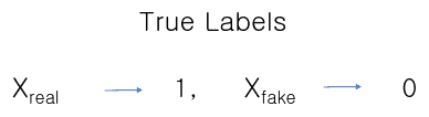
Next, the predictions are compared with the ground truth { 0: fake, 1: real }, and a Binary Cross-Entropy (BCE) loss is calculated.
The loss (or gradient) is then backpropagated only through the discriminator, and its parameters are optimized accordingly.

In the second step,

The generator produces images X_fake , which are again passed through the discriminator.
Here too it outputs a prediction Y_pred.
And the BCE loss is computed.
Now, in this alternate step, because you want to enforce your Generator to produce images, as similar to the real images as possible (i.e., close to the true distribution), the true labels (or ground truth) are all labeled as ‘real’ or 1. As a result, when the generator tries to fool the discriminator (into believing that the images generated by it are real), the loss is backpropagated only through the generator network, and its parameters are optimized suitably.

Image showing the training procedure of GANs.what is a generative adversarial network — Figure 10: The training procedure of Generative Adversarial Networks.

It is important to note that for the generator to produce realistic images, the discriminator has to guide (loss for fake images are backpropagated through the generator). Thus, there is a need for both networks to be strong enough. If:

The discriminator is a weak classifier, so even non-plausible images produced by the generator will be classified as real. The end result is that the generator produces low-quality images.
The generator is weak; it will not be able to fool the discriminator, as it will not generate images similar to the true distribution.

Objective Function of GAN

The generator and the discriminator you have seen are trained, based on the classification score given by the discriminator’s final layer, telling how fake or real its input had been. Surely that makes cross-entropy function the obvious choice when training such a network. We are dealing with a binary-class classification problem here, so a Binary Cross-Entropy (BCE) function is used.

(1) $\begin{equation*}L(\hat{y}, y) = -\frac{1}{N}\sum_{i=1}^{N}\left[ y_i \log\hat{y_i} + (1-y_i) \log (1-\hat{y_i}) \right]\end{equation*}$

binary_cross_entropy = tf.keras.losses.BinaryCrossentropy()

In the eq. 1, you can see the complete BCE loss function. Let’s break down the above equation and understand the various components of it.

The negative sign at the beginning of the equation is there to avoid the loss from being negative. As the neural-network output is normalized between $0$ and $1$ , taking $log$ of values in this range would result in a value less than zero. Hence, we solve the negative log-likelihood.
Remember that we train our neural network in batches. The summation from $1$ to $N$ means that your loss is computed for the N training samples per batch, and you then take the average of those samples by dividing it by $N$ ( batch ). In short, average the loss across the batch.
The $\hat{y_i}$ is the prediction made by the model or discriminator in GAN, while the $y_i$ is the true label, irrespective of the sample being real ( 0 ) or fake ( 0 ).
Did you note that there are two terms in the loss function, but only one is relevant? That’s because the first term is valid when the true label is $1$ ( real ), and the second is valid when the true label is $0$ ( fake ).

Now that you have understood the BCE loss function see how it is modeled in Generative Adversarial Networks.

The generator aims to learn a distribution $p_g$ over original data $x$ .
A prior is defined on input noise variables $p_z(z)$ sampled from the normal distribution.
Then the input noise vector is mapped to a data space as $G(z; θ_g )$ , where $G$ is a differentiable function, represented by a stack of fully-connected networks with learnable parameters $\theta_{g}$ .
A second fully-connected network $D(x;$ $\theta_d)$ outputs a single scalar value $[0, 1]$ . $D(x)$ represents the probability that $x$ came from the true data distribution rather than $p_g$ or generator $G$ . The network is trained to maximize the probability of $D$ assigning the correct label to both training examples and samples produced from $G$ .
At the same time, we train $G$ to minimize $-log(1- D(G(z)))$ .

In other words, $D$ and $G$ play the following two-player minimax game with value function $V (G, D)$ :

(2) $\begin{equation*}$min_{G}max_{D}V (D, G) = E_{x \sim p_{data}(x)}[log D(x)] + E_{z \sim p_{z}(z)}[log(1-D(G(z)))]$ \end{equation*}$

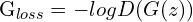
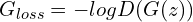
As observed in the paper of GAN, Eq. 2 may not provide sufficient gradient for the generator to learn well. Training this way will achieve only half the objective. Though the discriminator definitely becomes more powerful, for it can now easily discriminate the real from the fake, the generator lags behind. It has still not learned to produce realistic-looking images.

Early in learning, when $G$ is poor, $D$ can reject samples with high confidence because they are clearly different from the training data. In this case, $-log(1 - D(G(z)))$ saturates. Hence, rather than training $G$ to minimize $-log(1 - D(G(z)))$ , they train $G$ to maximize $-log D(G(z))$ .

Next, let’s examine the above objective function in greater detail.

The discriminator is a binary classifier that, given an input $x$ , outputs a probability $D(x)$ between 0 and 1.

generative adversarial networks tutorial

As the true label for $X_{real}$ is 1 and the true label for $X_{fake}$ is 0:

The probability $D(x)$ closer to 1 means that the discriminator predicts the input is an actual image.
And a probability closer to 0 means that the input is fake.

advantages of generative adversarial networks

Assuming the role of a mentor or the police, the discriminator says yes to only what is right, the goal is to classify $X_{real}$ as real and $X_{fake}$ as fake.

Thus, the objective of the discriminator becomes:

Maximizing the probability $D(X_{real})$ i.e. bringing it closer to 1

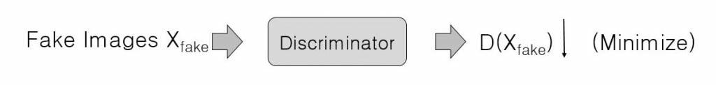
Minimizing the probability $D(X_{fake})$ , where $X_{fake}$ is $G(Z)$

generative adversarial networks explained

To model the objective of the generator and the discriminator, we will use the Binary Cross-Entropy loss function from equation 1.

For the first objective of the discriminator, i.e. to maximize the probability $D(X_{real})$ : the true label $y$ is 1, and the predicted output $\hat{y}$ is $D(X_{real})$ . Putting these values in the BCE loss function equation 1, we get:

(3) $\begin{equation*}$D_{loss_{real}} = - log D(X_{real})$\end{equation*}$

# y_hat = D(X_real), y = 1
D_loss_real = binary_cross_entropy(tf.ones_like(y), D(X_real))

For the second objective, i.e., to minimize the probability $D(X_{fake})$ : the true label $y$ is 0, and the predicted output $\hat{y}$ is $D(X_{fake})$ , where $X_{fake}$ is equal to $G(z)$ . Putting these values in the BCE loss function, we get:

(4) $\begin{equation*}$D_{loss_{fake}} = - log (1 - D(G(z))$\end{equation*}$

# y_hat = D(X_fake), X_fake = G(z), y = 0
D_loss_fake = binary_cross_entropy(tf.zeros_like(y), D(X_fake))

Therefore, the cumulative Discriminator loss becomes:

(5) $\begin{equation*}$D_{loss} = D_{loss_{real}} + D_{loss_{fake}}$\end{equation*}$

(6) $\begin{equation*}$D_{loss} = - log D(X_{real}) - log (1 - D(G(z))$\end{equation*}$

def discriminator_loss(D(X_real), D(X_fake)):
    D_loss_real = binary_cross_entropy(tf.ones_like(D(X_real)), D(X_real))
    D_loss_fake = binary_cross_entropy(tf.zeros_like(D(X_fake)), D(X_fake))
    D_loss = D_loss_real + D_loss_fake
    return D_loss

Now, the generator wants the images generated by it to be classified as real by the discriminator.

Thus, the objective of the generator becomes:

Maximizing the probability $D(G(z)$ i.e. bringing it closer to 1.

For this objective, i.e., to maximize the probability $D(G(z))$ by the discriminator, the true label $y$ is 1, and the predicted output $\hat{y}$ is $D(G(z))$ . Putting these values in the BCE loss function, we get:

(7) $\begin{equation*}$G_{loss} = - log D(G(z))$\end{equation*}$

# y_hat = D(G(z)),  y = 1
def generator_loss(D(G(z))):
    G_loss = binary_cross_entropy(tf.ones_like(D(G(z))), D(G(z))) 
    return G_loss

Now, let’s look at the Minibatch stochastic gradient descent training of generative adversarial nets. The number of steps to apply to the discriminator, $k$ , is a hyperparameter. A value of $k = 1$ is used, as it is the least expensive option.

for number of training, iterations do
    for  steps do
        1. Sample minibatch of  noise samples  
           from noise prior .
        2. Sample minibatch of  examples    
           from data generating distribution .  
        3. Update the discriminator by minimizing the 
           Discriminator loss,   
    end for 
    1. Sample minibatch of  noise samples 
       from noise prior .
    2. Update the generator by minimizing the Generator loss,
           
end for

You know enough about the GAN and its functions by now to move on to coding a GAN to generate images.

Coding a Vanilla GAN in a Few Lines

Here, we will code a GAN using both Pytorch and Tensorflow frameworks. You will learn to generate images related to Fashion categories from noise vectors.

Dataset

We will use the famous Fashion-MNIST dataset for this purpose.

The Fashion-MNIST dataset consists of:

Database of 60,000 fashion images is shown on the right.
Each image of size 28×28 ( grayscale ) is associated with a label from 10 categories like t-shirts, trousers, sneakers, etc.

To learn more about the dataset, like class distribution, data curation, and benchmark comparison, please check out their Github repository.

In this experiment, we will only use the training split of this dataset, which contains 60,000 images.

Images from this dataset will be the real images that we have been talking about throughout this post. Once trained, our generator will be able to generate realistic fashion images, quite like the ones shown above.

Note: Pytorch and Tensorflow implementations were carried out on a 16GB Pascal 100 GPU.

Download Code To easily follow along this tutorial, please download code by clicking on the button below. It's FREE!

Click here to download the source code to this post

Pytorch Implementation

Importing Modules

# import the required packages
import torch
import argparse
import numpy as np
import torch.nn as nn
import torch.optim as optim
from torchvision import datasets, transforms
from torch.autograd import Variable
from torchvision.utils import save_image
from torchvision.utils import make_grid
from torch.utils.tensorboard import SummaryWriter

# construct the argument parser
parser = argparse.ArgumentParser()
parser.add_argument("--n_epochs", type=int, default=200, help="number of epochs of training")
parser.add_argument("--batch_size", type=int, default=128, help="size of the batches")
parser.add_argument("--lr", type=float, default=2e-4, help="adam: learning rate")
parser.add_argument("--b1", type=float, default=0.5, help="adam: decay of first order momentum of gradient")
parser.add_argument("--b2", type=float, default=0.999, help="adam: decay of first order momentum of gradient")
parser.add_argument("--latent_dim", type=int, default=100, help="dimension of the latent space (generator's input)")
parser.add_argument("--img_size", type=int, default=28, help="image size")
parser.add_argument("--channels", type=int, default=1, help="image channels")
args = parser.parse_args()

We begin with importing necessary packages like Torch, Torchvision, and numpy on Lines 2-11. In today’s tutorial, you need Torch 1.6 and Torchvision 0.7 with Cuda 10.1. The code can be reproduced without any installations on Google Collaborator.

From Lines 14-23 we parse the command line arguments:

--n_epochs: Number of epochs you train the model.
--batch_size: Number of images passed to the model in each forward pass.
--lr: Learning rate of the network.
--b1 and --b2: Decay of the first-order momentum of gradients for adam optimizer.
--latent_dim: The dimensionality of the noise vector fed to the generator as input.
--img_size: Size of the image for each dimension.
--channels: Number of channels in the image ( grayscale: 1, rgb: 3 ).

Loading and Preprocessing Dataset

train_transform = transforms.Compose([
    transforms.ToTensor(),
    transforms.Normalize(mean=(0.5), std=(0.5))])

train_dataset = datasets.FashionMNIST(root='./data/', train=True, transform=train_transform, download=True)

train_loader = torch.utils.data.DataLoader(dataset=train_dataset, batch_size=args.batch_size, shuffle=True)

In Lines 24-26,

You pass a list of transforms to be composed. The images are normalized using the mean and standard deviation of 0.5. Note that there is one value for both, as we are dealing with a grayscale image here. The normalization maps pixel values from [0, 255] to [-1, 1]. The range [-1, 1] is preferred, having proven useful for training GANs (Generative Adversarial Networks)
You also convert the images to tensors.

Next, in Line 28, you load the Fashion-MNIST training data and apply the train_transform ( normalization and converting images to tensors ). The best part is that you can load the Fashion-MNIST dataset on the fly using Pytorch’s dataset module.

Line 30 defines the training data loader, which combines the Fashion-MNIST dataset and provides an iterable over the given dataset. Here you will specify the batch_size (How many images in each batch ) and, shuffle = True which will reshuffle the data after every epoch.

Generator Network

# Generator Model Definition
class Generator(nn.Module):
    def __init__(self):
        super(Generator, self).__init__()

        self.model = nn.Sequential(nn.Linear(noise_vector, 128),
        							nn.LeakyReLU(0.2, inplace=True),
        							nn.Linear(128, 256),
                      nn.BatchNorm1d(256, 0.8),
        							nn.LeakyReLU(0.2, inplace=True), 
        							nn.Linear(256, 512),
                      nn.BatchNorm1d(512, 0.8),
        							nn.LeakyReLU(0.2, inplace=True), 
                      nn.Linear(512, 1024),
                      nn.BatchNorm1d(1024, 0.8),
        							nn.LeakyReLU(0.2, inplace=True), 
        							nn.Linear(1024, image_dim),
        							nn.Tanh())
    
    def forward(self, noise_vector): 
        image = self.model(noise_vector)
        image = image.view(image.size(0), *image_shape)
        return image

In Lines 36-48, you define the generator’s sequential model, and the above model structure is quite intuitive. The Generator is a fully connected network that takes a noise vector ( latent_dim ) as an input and outputs a 784-dimensional vector. Consider the generator as a decoder fed with a low-dimensional vector ( 100-d ) and outputs an upsampled high-dimensional vector ( 784-d ).

The network mainly consists of dense layers, leakyrelu & tanh activation function and batchnorm1d layers.

The first layer has 128 neurons, doubled at every new linear layer, up to 1024 neurons.
Leaky ReLU has been used as the activation function in this network for the intermediate layers with a negative slope as $0.2$ , meaning the features with a value below $-0.2$ will be squashed to $0$ .
BatchNorm1d is also used to normalize the intermediate feature vectors with an eps of 0.8 for numerical stability. Default: 1e-5.
The tanh activation at the output layer ensures that the pixel values are mapped in line with its own output, i.e., between $(-1, 1)$ ( remember, we normalized the images to range $[-1, 1]$ ).

In Lines 50-53, the forward the function of the generator feeds the noise vector (normal distribution) to the model, then reshapes the 784-d vector to (1, 28, 28), the original image shape, and finally, the image is returned. The generator, as we know, mimics the real data distribution without actually seeing it.

Discriminator Network

# Discriminator Model Definition
class Discriminator(nn.Module):
    def __init__(self):
        super(Discriminator, self).__init__()

        self.model = nn.Sequential(nn.Linear(image_dim, 512),
        							nn.LeakyReLU(0.2, inplace=True),
        							nn.Linear(512, 256),
        							nn.LeakyReLU(0.2, inplace=True),
        							nn.Linear(256, 1),
        							nn.Sigmoid())
    
    def forward(self, image):
        image_flattened = image.view(image.size(0), -1)
        result = self.model(image_flattened)
        return result

The discriminator is a binary classifier consisting of only fully-connected layers. It is a simpler model with less layers than the generator. Lines 59-64 define the sequential-discriminator model:

Inputs the flattened image of dimension 784, and outputs a score between 0 and 1.
Has Leaky Relu in the intermediate layers
Has the Sigmoid activation function in the output layer

The forward function of the discriminator, Lines 66-69 flattens the input feeds from the vector to the discriminator, and returns the result, indicating whether the image is real or fake.

device = torch.device('cuda' if torch.cuda.is_available() else 'cpu')
generator = Generator().to(device)
discriminator = Discriminator().to(device)

Line 70 defines the device Torch shall use while you train your network. And in Lines 71-72, both generator and discriminator models are moved to a device, which can be CPU or GPU, depending on the hardware.

Loss function

adversarial_loss = nn.BCELoss()

As mentioned earlier, the Binary Cross-Entropy loss helps model the objectives of the two networks.

Optimization

G_optimizer = optim.Adam(generator.parameters(), lr=args.lr, betas=(args.b1, args.b2)
D_optimizer = optim.Adam(discriminator.parameters(), lr=args.lr, betas=(args.b1, args.b2)

The generator and discriminator are optimized with Adam optimizer.

The generator and discriminator are both optimized with the Adam optimizer. Three arguments are passed to the optimizer:

Generator and discriminator parameters, or weights to be optimized
A learning rate of
Betas coefficients b1 & b2 for computing running averages of gradient during backpropagation

Training the networks

Discriminator

The discriminator is trained on both real and fake images.

for epoch in range(1, args.n_epochs+1): 

    D_loss_list, G_loss_list = [], []

    for index, (real_images, _) in enumerate(train_loader):
      
      D_optimizer.zero_grad() # zero-out the old gradients 
      real_images = real_images.to(device)
      real_target = Variable(torch.ones(real_images.size(0), 
                    1).to(device))
      fake_target= Variable(torch.zeros(real_images.size(0), 
                   1).to(device))
      # Training Discriminator on Real Data
      D_real_loss = 
                adversarial_loss(discriminator(real_images), 
                real_target)
      
      # noise vector sampled from a normal distribution 
      noise_vector = 
                   Variable(torch.randn(real_images.size(0), 
                   args.latent_dim).to(device))
      noise_vector = noise_vector.to(device)
      generated_image = generator(noise_vector)

      # Training Discriminator on Fake Data
      D_fake_loss = 
            adversarial_loss(discriminator(generated_image), 
            fake_target)

      D_total_loss = D_real_loss + D_fake_loss
      D_loss_list.append(D_total_loss)
      D_total_loss.backward()
      D_optimizer.step()

The training of the discriminator is done in two parts: real images and fake images (produced by generator). As we process the batches in the dataset, the discriminator classifies images as real or fake. It has two losses: real loss and fake loss. Added up, they give the combined loss (you could even take the average of the two losses), which is used to optimize the discriminator’s weights.

In Lines 90-92, the discriminator classifies the real images and calculates the BCE loss D_real_loss, against the real targets you created in Lines 84-85.

In Lines 95-97, you sample the noise vector noise_vector from a normal distribution with a mean of 0 and a standard deviation of 1. The noise_vector has a dimension of $(128 , 100)$ . Lines 102-104 feeds the fake images and calculate the BCE loss D_fake_loss against the fake targets created in Lines 86-87.

Finally, you add the two losses, compute the gradients D_total_loss.backwards(), and optimize the discriminator’s parameters with D_optimizer.step().

Generator

The generator is trained with feedback from the discriminator.

# Train G on D's output
        G_optimizer.zero_grad() # zero out the old gradients
        generated_image = generator(noise_vector)
        G_loss = 
            adversarial_loss(discriminator(generated_image), 
            real_target) # G tries to dupe the discriminator
        G_loss_list.append(G_loss)
        G_loss.backward()
        G_optimizer.step()

The generator also generates images from a latent variable vector and updates its parameters using the generator loss. In Line 110,

You feed the noise vector to the generator, which produces the fake generated_image.
Next, you pass on the generated_image to the discriminator for classification.

Note: The adversarial_loss is calculated with labels as real_target ( 1 ), as you would like the generator to fool the discriminator and produce real images.

Finally, G_loss.backward() computes the gradients and G_optimizer.step() optimizes the generator’s parameters.

Discriminator and Generator Loss Plot

The image shows the loss curves for the generator and discriminator after training the GAN. introduction to generative adversarial networks — Figure 16. The Generator and Discriminator loss curves after training.

From the above loss curves, it is evident that the discriminator loss is initially low while the generators is high. However, as training progresses, we see that the generator’s loss decreases, meaning it produces better images and manages to fool the discriminator. Consequently, the discriminator’s loss increases. But of course, you cannot expect a smooth graph. Around the ~80th epoch, you find the generator’s loss rising again, which could be due to various factors. One reason is, as the discriminator is trained, it changes the loss landscape of the generator. It could also signal that the training ends here, at this ~80th epoch, and the generator cannot be improved anymore beyond this epoch.

Results

Look at the three images below. The generator produced them at three different stages of the training. You can clearly see that initially, the generator is producing noisy images. But as the training progresses, it starts generating more realistic-looking fashion images.

Images generated by the generator during training. advantages and disadvantages of gan — Figure 17. Image generated by the generator at three different stages of training.

Tensorflow Implementation

Let’s reproduce the Pytorch implementation of GAN in Tensorflow. For this implementation, we would use Tensorflow v2.3.0 and Keras v2.4.3.

Importing the Packages

#import the required packages
import os
import time
import tensorflow as tf
from tensorflow.keras import layers
from IPython import display
import matplotlib.pyplot as plt
%matplotlib inline

# construct the argument parser
parser = argparse.ArgumentParser()
parser.add_argument("--n_epochs", type=int, default=200, help="number of epochs of training")
parser.add_argument("--batch_size", type=int, default=128, help="size of the batches")
parser.add_argument("--lr", type=float, default=2e-4, help="adam: learning rate")
parser.add_argument("--b1", type=float, default=0.5, help="adam: decay of first order momentum of gradient")
parser.add_argument("--b2", type=float, default=0.999, help="adam: decay of first order momentum of gradient")
parser.add_argument("--latent_dim", type=int, default=100, help="dimension of the latent space (generator's input)")
parser.add_argument("--img_size", type=int, default=28, help="image size")
parser.add_argument("--channels", type=int, default=1, help="image channels")
args = parser.parse_args()

We begin by importing the necessary packages like TensorFlow, TensorFlow layers, time, and matplotlib to plot on Lines 2-10.

From Lines 11-20, we parse the command line arguments like epochs, image size, batch size, etc.

Next, we move on to loading and preprocessing of the Fashion-MNIST dataset.

Data Loading and Preprocessing

(x_train, y_train), (x_test, y_test) = tf.keras.datasets.fashion_mnist.load_data()
x_train = x_train.reshape(x_train.shape[0], 28, 28, 1).astype('float32')
x_train = (x_train - 127.5) / 127.5 # Normalize the images to [-1, 1]
# Batch and shuffle the data
train_dataset = tf.data.Dataset.from_tensor_slices(x_train).\
shuffle(60000).batch(args.batch_size)

Loading the dataset is fairly simple; you can use the tf_keras datasets module, which loads the data off the shelf. Since we do not require the labels to solve this problem, we will use the training images x_train. In Line 22, you reshape the images and cast them to float32 since the data is inherently in uint8 format.

Then, in Line 23, you normalize the data from [0, 255] to [-1, 1]. Finally, we build the TensorFlow input pipeline, which is similar in spirit to PyTorch data loaders. In short, tf.data.Dataset.from_tensor_slices is fed the training data, shuffled, and sliced into tensors, allowing you to access tensors of specified batch size during training. The buffer size parameter in shuffle affects the randomness of the shuffle.

Define the Generator Network

def generator(image_dim):
    
    inputs = layers.Input(shape=(100,))
    x = layers.Dense(128, kernel_initializer=tf.keras.initializers.he_uniform)(inputs)
    print(x.dtype)
    x = layers.LeakyReLU(0.2)(x)
    x = layers.Dense(256, kernel_initializer=tf.keras.initializers.he_uniform)(x) 
    x = layers.BatchNormalization(momentum=0.1,  epsilon=0.8)(x)
    x = layers.LeakyReLU(0.2)(x)
    x = layers.Dense(512, kernel_initializer=tf.keras.initializers.he_uniform)(x) 
    x = layers.BatchNormalization(momentum=0.1,  epsilon=0.8)(x)
    x = layers.LeakyReLU(0.2)(x)
    x = layers.Dense(1024, kernel_initializer=tf.keras.initializers.he_uniform)(x) 
    x = layers.BatchNormalization(momentum=0.1,  epsilon=0.8)(x)
    x = layers.LeakyReLU(0.2)(x)
    x = layers.Dense(image_dim, activation='tanh', kernel_initializer=tf.keras.initializers.he_uniform)(x) 
    outputs = tf.reshape(x, [-1, args.img_size, args.img_size, args.channels], name=None)
    model = tf.keras.Model(inputs, outputs, name="Generator")
    return model

Be it TensorFlow or PyTorch, the architecture of the generator remains exactly the same as above. You do need to modify the generator function though.

The generator is fed a 100-d noise vector, sampled from a normal distribution. In Line 29,

We define the input layer, with shape as (100,).
The PyTorch Linear layers are replaced by Tensorflow’s Dense layers.
In PyTorch, the default weight initializer for the linear layers is kaiming_uniform. TensorFlow uses he_uniform, which is very similar.
The momentum value of the batch norm layers is changed to 0.1 (default is 0.99).

In Line 43, we reshape the 784-d tensor to (Batch Size, 28, 28, 1) using tf.reshape in which the first parameter is the input tensor, and the second parameter is the new shape of the tensor. Finally, we create the Model by passing the generator function’s input and output layers ( Line 44 ).

Image of the generator neural network. — Figure 18. The generator network.

Discriminator Function

def discriminator():
    inputs = layers.Input(shape=(args.img_size, args.img_size, args.channel))
    reshape = tf.reshape(inputs, [-1, 784], name=None)
    x = layers.Dense(512, kernel_initializer=tf.keras.initializers.he_uniform)(reshape)
    x = layers.LeakyReLU(0.2)(x)
    x = layers.Dense(256, kernel_initializer=tf.keras.initializers.he_uniform)(x) 
    x = layers.LeakyReLU(0.2)(x)
    outputs = layers.Dense(1, activation='sigmoid', kernel_initializer=tf.keras.initializers.he_uniform)(x) 
    model = tf.keras.Model(inputs, outputs, name="Discriminator")
    return model

Keep in mind that the discriminator is a binary classifier consisting only of fully -connected layers. So, the discriminator expects a tensor of shape (Batch Size, 28, 28, 1). But the discriminator function consists of only dense layers. We, therefore, in Line 48, need to reshape the tensor to a vector of shape (Batch Size, 784) .

The final layer has the sigmoid activation function, which squashes the output value between 0 (fake) and 1 (real).

The image on the right represents the discriminator network architecture. Check it out for more insights into the network layout.

Loss Function

adversarial_loss = tf.keras.losses.BinaryCrossentropy()

Define the Binary Cross-Entropy loss to model the two networks’ objectives.

gan advantages and disadvantages — Figure 19. Discriminator network.

Generator Loss

def generator_loss(fake_output):
    gen_loss = adversarial_loss(tf.ones_like(fake_output), fake_output)
    #print(gen_loss)
    return gen_loss

The generator_loss function is fed the fake outputs produced by the discriminator, as the input to the discriminator was fake images (produced by the generator).

Note: The generator_loss is calculated with labels as real_target ( 1 ) because you want the generator to fool the discriminator and produce real images.

Discriminator Loss

def discriminator_loss(real_output, fake_output):
    real_loss = adversarial_loss(tf.ones_like(real_output), real_output)
    fake_loss = adversarial_loss(tf.zeros_like(fake_output), fake_output)
    total_loss = real_loss + fake_loss
    #print(total_loss)
    return total_loss

The discriminator loss is the sum of real and fake loss for its job is to differentiate between real images and those generated by the generator. Unlike the generator loss, here:

the real (original images) output predictions label is 1
fake output predictions label is 0

Optimizer

generator_optimizer = tf.keras.optimizers.Adam(lr = args.lr, beta_1 = args.b1, beta_2 = args.b2 )
discriminator_optimizer = tf.keras.optimizers.Adam(lr = args.lr, beta_1 = args.b1, beta_2 = args.b2 )

Both generator and discriminator are optimized with the Adam optimizer. Two arguments are passed to it:

a learning rate of $2e-4$ ,
betas coefficients b1 & b2

These compute the running averages of gradients during backpropagation.

Training the Discriminator and Generator Network

@tf.function
def train_step(images):
    noise = tf.random.normal([args.batch_size, args.latent_dim])

    with tf.GradientTape() as gen_tape, tf.GradientTape() as disc_tape:
      generated_images = generator(noise, training=True)

      real_output = discriminator(images, training=True)
      fake_output = discriminator(generated_images, training=True)
      
      gen_loss = generator_loss(fake_output)
      disc_loss = discriminator_loss(real_output, fake_output)
      
    
    gradients_of_gen = gen_tape.gradient(gen_loss, generator.trainable_variables) # computing the gradients


    gradients_of_disc = disc_tape.gradient(disc_loss, discriminator.trainable_variables) # computing the gradients
    

    generator_optimizer.apply_gradients(zip(gradients_of_gen, generator.trainable_variables))#updating generator parameter  

    
    discriminator_optimizer.apply_gradients(zip(
gradients_of_disc,discriminator.trainable_variables))#updating discriminator parameter

The train_step function is the core of the whole GAN training. For this is where you combine all the training functions defined above. Note the use of @tf.function in Line 101, this compiles the train_step function into a callable TensorFlow graph. Also, speeds up the training time (check this out for yourself).

In the training loop,

First, we sample the noise from a normal distribution and input it to the generator.
The generator model then produces an image.
We start by feeding the discriminator model real images. Then also input images produced by the generator model, which are classified as either real images (drawn from the training set) or fakes (produced by the generator).
The loss is calculated for each of these models: gen_loss and disc_loss.
After computing the gradients, the generator and discriminator parameters are updated using the Adam optimizer.

def train(dataset, epochs):
  for epoch in range(epochs):
    start = time.time()
    for image_batch in dataset:
      train_step(image_batch)

    print ('Time for epoch {} is {} sec'.format(epoch + 1, time.time()-start))


train(train_dataset, args.epoch)

Finally, it’s time to train our first GAN model in Tensorflow. Taking the train_dataset and Epochs as the parameters, the above train function calls the train_step function, at every new batch, in total (Total Training Images / Batch Size). The training is pretty fast. Each epoch takes around 2-3 seconds to train on a Pascal 100 GPU.

Results

Look at the three image grids below. Each of these grids consists of 16 images, and was produced by the generator, at three different stages of the training. As in Pytorch implementation, you can see that initially, the generator produces noisy images. But as training progresses, the generator starts producing more realistic-looking fashion images..

Image generated by the generator at three different stages of training. GANS — Figure 20. Image generated by the generator at three different stages of training.

Self-supervised learning is an elegant subset of unsupervised learning, where you can generate output labels ‘intrinsically’ from data objects by exposing a relation between object parts or different views of the object.

Summary

We started by discussing why we need GANs, their advantages, and the intuition behind them.
Then we dug deeper and introduced you to the components that make a GAN, i.e., the generator and discriminator.
We then discussed in detail the two most important aspects: The training Strategy and the Objective Function of GAN
Finally, we implemented a Vanilla GAN, in both Pytorch and TensorFlow framework, with the Fashion-MNIST dataset and achieved comparable results.

References

Was This Article Helpful?

TRM: Tiny AI Models beating Giants on Complex Puzzles

Models with billions, or trillions, of parameters are becoming the norm. These models can write

Deploying ML on Arduino: From Blink to Think

Deploying ML on Arduino Nano 33 BLE. Explore TinyML techniques, setup steps, and why older

VideoRAG: Redefining Long-Context Video Comprehension

Discover VideoRAG, a framework that fuses graph-based reasoning and multi-modal retrieval to enhance LLMs’ ability

Was This Article Helpful?

VideoRAG: Redefining Long-Context Video Comprehension

Discover VideoRAG, a framework that fuses graph-based reasoning and multi-modal retrieval to enhance LLMs' ability to understand multi-hour videos efficiently.

AI Agent in Action: Automating Desktop Tasks with VLMs

Agentic AIGUIVLMs

Kukil September 30, 2025

AI Agent in Action: Automating Desktop Tasks with VLMs

Learn how to build AI agent from scratch using Moondream3 and Gemini. It is a generic task based agent free from…

The Ultimate Guide To VLM Evaluation Metrics, Datasets, And Benchmarks

Computer VisionVLMs

Bhomik Sharma September 23, 2025

The Ultimate Guide To VLM Evaluation Metrics, Datasets, And Benchmarks

Get a comprehensive overview of VLM Evaluation Metrics, Benchmarks and various datasets for tasks like VQA, OCR and Image Captioning.

Subscribe to our Newsletter

Subscribe to our email newsletter to get the latest posts delivered right to your email.

Generative Adversarial Networks (GANs) – An Introduction

What are Generative Adversarial Networks (GANs)?

Why Generative Adversarial Networks(GANs)?

Advantages of GANs Over Other Generative Models

Intuition Behind Generative Adversarial Networks(GANs)

Components of a GAN

Generator

Discriminator

Training Procedure

Objective Function of GAN

Coding a Vanilla GAN in a Few Lines

Dataset

Pytorch Implementation

Importing Modules

Loading and Preprocessing Dataset

Generator Network

Discriminator Network

Loss function

Optimization

Training the networks

Discriminator

Generator

Discriminator and Generator Loss Plot

Results

Tensorflow Implementation

Importing the Packages

Data Loading and Preprocessing

Define the Generator Network

Discriminator Function

Loss Function

Generator Loss

Discriminator Loss

Optimizer

Training the Discriminator and Generator Network

Results

Summary

References

TRM: Tiny AI Models beating Giants on Complex Puzzles

Deploying ML on Arduino: From Blink to Think

VideoRAG: Redefining Long-Context Video Comprehension

Table of Contents

Read Next

VideoRAG: Redefining Long-Context Video Comprehension

AI Agent in Action: Automating Desktop Tasks with VLMs

The Ultimate Guide To VLM Evaluation Metrics, Datasets, And Benchmarks

Subscribe to our Newsletter

Subscribe to receive the download link, receive updates, and be notified of bug fixes

Which email should I send you the download link?

Get Started with OpenCV