


Photography is the favorite hobby of millions of people around the world. After all, how difficult can it be! In the words of Diane Arbus, a famous American photographer —
“Taking pictures is like tiptoeing into the kitchen late at night and stealing Oreo cookies.”
Taking a photo is easy, but taking a high-quality photo is hard. It requires good composition and lighting. The right lens and superior equipment can make a big difference. But above all, a high-quality photo requires good taste and judgment. You need an eye of an expert.
But is there a mathematical quality measure that captures this human judgment?
The answer is both yes and no!
There are some measures of quality that are easy for an algorithm to capture. For example, we can look at the information captured by the pixels and flag an image as noisy or blurry.
On the other hand, some measures of quality are almost impossible for an algorithm to capture. For example, an algorithm would have a tough time assessing the quality of a picture that requires cultural context.
In this post, we will learn about an algorithm for predicting image quality score.
Note: This tutorial has been tested on Ubuntu 18.04, 16.04, with Python 3.6.5, Python 2.7 and OpenCV 3.4.1 and 4.0.0-pre versions.
What is Image Quality Assessment (IQA)?
Image Quality Assessment (IQA) algorithms take an arbitrary image as input and output a quality score as output. There are three types of IQAs:
- Full-Reference IQA: Here you have a ‘clean’ reference (non-distorted) image to measure the quality of your distorted image. This measure may be used in assessing the quality of an image compression algorithm where we have access to both the original image and its compressed version.
- Reduced-Reference IQA: Here you don’t have a reference image, but an image having some selective information about it (e.g. watermarked image) to compare and measure the quality of distorted image.
- Objective Blind or No-Reference IQA: The only input the algorithm gets is the image whose quality you want to measure. This is thus called, No-Reference or Objective-Blind.


No-Reference IQA
In this post, we will discuss one of the No-Reference IQA Metrics, called Blind/Referenceless Image Spatial Quality Evaluator (BRISQUE). Before we go deeper into the theory, let’s first understand two basic terms:
- Distorted Image: As the name suggests, a distorted image is a version of the original image that is distorted by blur, noise, watermarking, color transformations, geometric transformations and so on and so forth.

As you can imagine, it is not always clear-cut whether an image is distorted or it’s natural. For example, when a video is smartly rendered with motion blur, the algorithm may get confused about its quality because of the intentional blur. So one has to use this quality measure in the right context.
Image Quality Assessment (IQA) Dataset
Quality is a subjective matter. To teach an algorithm about good and bad quality, we need to show the algorithm examples of many images and their quality score.
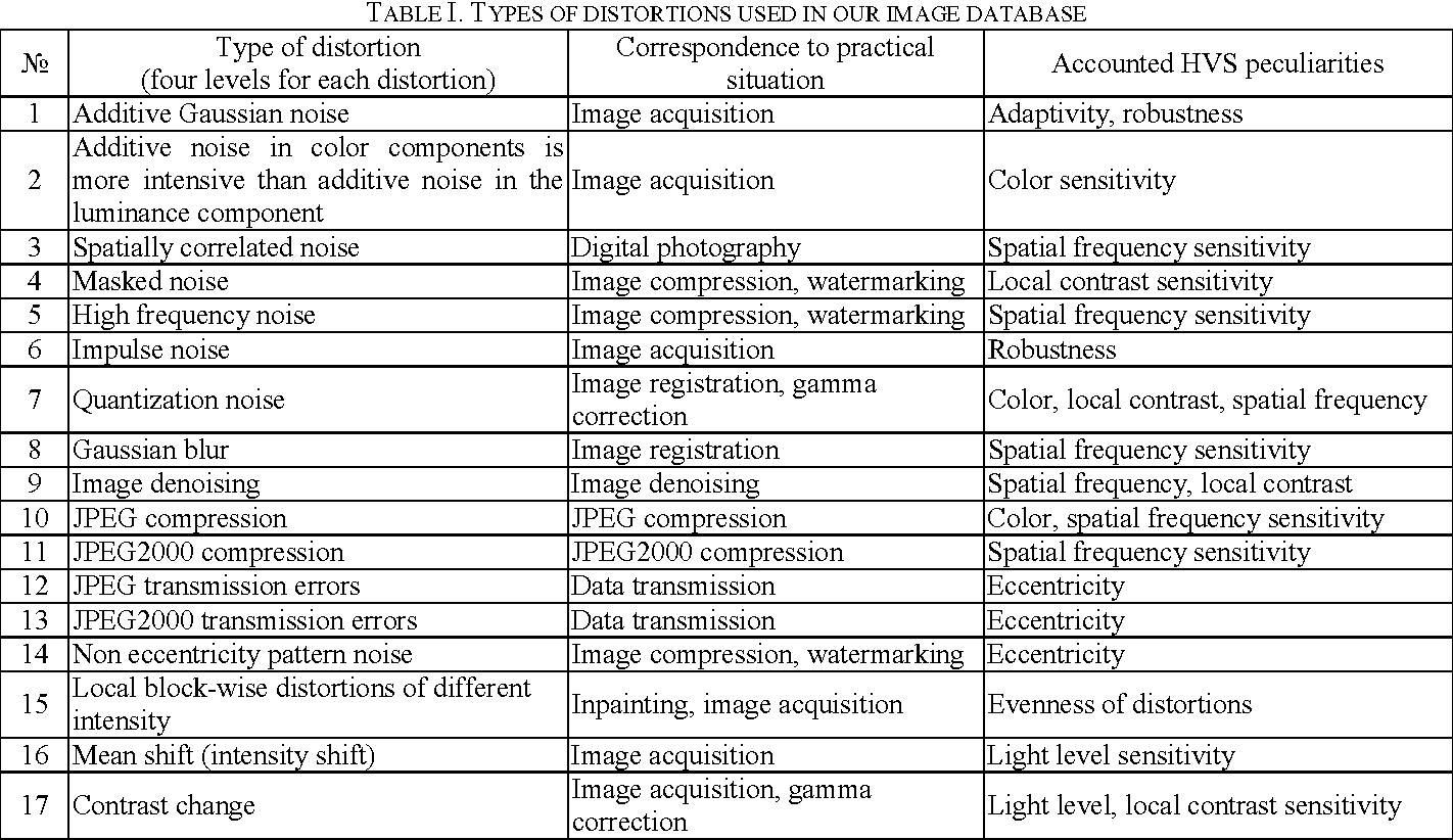
Who assigns the quality score for these training images? Humans, of course. But we cannot rely on the opinion of just one human. So we need opinions of several humans and assign the image a mean score between 0 (best) and 100 (worst). This score is called the Mean Quality Score in academic literature.
Do we need to collect this data ourselves? Fortunately, this dataset called TID2008 has been made available for research purposes.
Blind/Referenceless Image Spatial Quality Evaluator (BRISQUE)
In this section, we will describe the steps needed for BRISQUE algorithm used for No-Reference IQA. We have modified the C++ code provided by the authors to work on OpenCV 3.4. In addition, we have written code for Python 2 and Python 3.
Fig. 5 shows the steps involved in calculating BRISQUE.

Step 1: Extract Natural Scene Statistics (NSS)
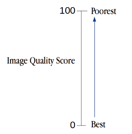
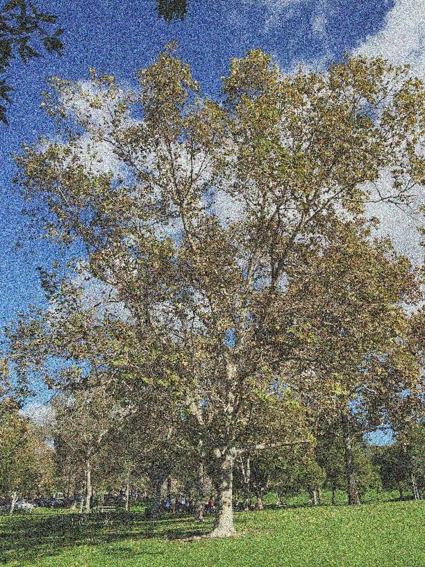
The distribution of pixel intensities of natural images differs from that of distorted images. This difference in distributions is much more pronounced when we normalize pixel intensities and calculate the distribution over these normalized intensities. In particular, after normalization pixel intensities of natural images follow a Gaussian Distribution (Bell Curve) while pixel intensities of unnatural or distorted images do not. The deviation of the distribution from an ideal bell curve is therefore a measure of the amount of distortion in the image.
We have shown this in the Figure below.
Mean Substracted Contrast Normalization (MSCN)
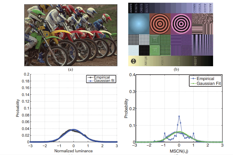
There are a few different ways to normalize an image. One such normalization is called Mean Substracted Contrast Normalization (MSCN). The figure below shows how to calculate MSCN coefficients.
This can be visualized as:
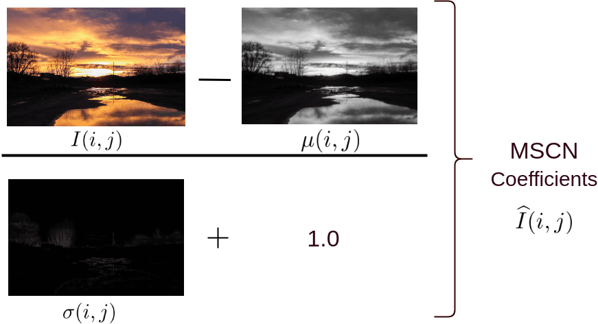
To calculate the MSCN Coefficients, the image intensity  at pixel
  is transformed to the luminance
  .
.
(1) 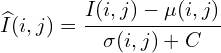
Where  (M and N are height and width respectively). Functions
  and
and  are local mean field and local variance field respectively. Local Mean Field (
 ) is nothing but the Gaussian Blur of the original image, while Local Variance Field (
 ) is the Gaussian Blur of the square of the difference of original image and . In the equation below
  is the Gaussian Blur Window function.
(2) 
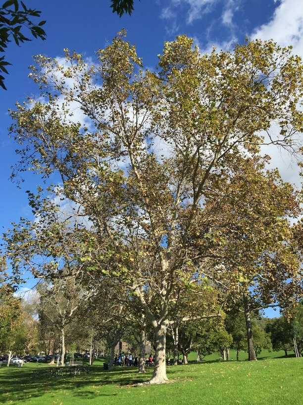
We use GaussianBlur function in C++ and Python to calculate MSCN Coefficients, as shown below:

C++
Mat im = imread("image_scenery.jpg"); // read image
cvtColor(im, im, COLOR_BGR2GRAY); // convert to grayscale

im.convertTo(im, 1.0/255); // normalize and copy the read image to orig_bw
Mat mu(im.size(), CV_64FC1, 1);
GaussianBlur(im, mu, Size(7, 7), 1.166); // apply gaussian blur
Mat mu_sq = mu.mul(mu);

// compute sigma
Mat sigma = im.size(), CV_64FC1, 1);
sigma = im.mul(im);
GaussianBlur(sigma, sigma, Size(7, 7), 1.166); // apply gaussian blur
subtract(sigma, mu_sq, sigma); // sigma = sigma - mu_sq
cv::pow(sigma, double(0.5), sigma); // sigma = sqrt(sigma)
add(sigma, Scalar(1.0/255), sigma); // to avoid DivideByZero Exception
Mat structdis(im.size(), CV_64FC1, 1);
subtract(im, mu, structdis); // structdis = im - mu
divide(structdis, sigma, structdis);
Python
im = cv2.imread("image_scenery.jpg", 0) # read as gray scale
blurred = cv2.GaussianBlur(im, (7, 7), 1.166) # apply gaussian blur to the image
blurred_sq = blurred * blurred
sigma = cv2.GaussianBlur(im * im, (7, 7), 1.166)
sigma = (sigma - blurred_sq) ** 0.5
sigma = sigma + 1.0/255 # to make sure the denominator doesn't give DivideByZero Exception
structdis = (im - blurred)/sigma # final MSCN(i, j) image
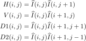
Pairwise products for neighborhood releationships
MSCN provides a good normalization for pixel intensities. However, the difference in natural vs. distorted images is not limited to pixel intensity distributions, but also the relationship between a pixel and its neighbors.
To capture neighborhood relationshiops the authors used pair-wise products of MSCN image with a shifted version of the MSCN image. Four orientations are used to find the pairwise product for the MSCN coefficients, namely: Horizontal (H), Vertical (V), Left-Diagonal (D1), Right-Diagonal (D2).
(3) 
Pair-wise products can be calculated in Python and C++ as below:
C++:
// declare shifting indices array
int shifts[4][2] = {{0, 1}, {1, 0}, {1, 1}, {-1, 1}};

// calculate pair-wise products for every combination of shifting indices
for(int itr_shift = 1; itr_shift <= 4; itr_shift++)
{
    int* reqshift = shifts[itr_shift - 1]; // the required shift index
    // declare shifted image
    Mat shifted_structdis(imdist_scaled.size(), CV_64F, 1);
    // BwImage is a helper class to create a copy of the image and create helper functions to access it's pixel values
    BwImage OrigArr(structdis);
    BwImage ShiftArr(shifted_structdis);
    // calculate pair-wise component for the given orientation
    for(int i = 0; i < structdis.rows; i++)
    {
        for(int j = 0; j < structdis.cols; j++) { if(i + reqshift[0] >= 0 && i + reqshift[0] < structdis.rows && j + reqshift[1] >= 0 && j + reqshift[1] < structdis.cols)
            {
                ShiftArr[i][j] = OrigArr[i + reqshift[0]][j + reqshift[1]];
            }f
            else
            {
                ShiftArr[i][j] = 0;
            }
        }
    }
    Mat shifted_new_structdis;
    shifted_new_structdis = ShiftArr.equate(shifted_new_structdis);
    // find the pairwise product
    multiply(structdis, shifted_new_structdis, shifted_new_structdis);
}
Python:
# indices to calculate pair-wise products (H, V, D1, D2)
shifts = [[0,1], [1,0], [1,1], [-1,1]]
# calculate pairwise components in each orientation
for itr_shift in range(1, len(shifts) + 1):
    OrigArr = structdis
    reqshift = shifts[itr_shift-1] # shifting index

    for i in range(structdis.shape[0]):
        for j in range(structdis.shape[1]):
            if(i + reqshift[0] >= 0 and i + reqshift[0] < structdis.shape[0] \ and j + reqshift[1] >= 0 and j  + reqshift[1] < structdis.shape[1]):
               ShiftArr[i, j] = OrigArr[i + reqshift[0], j + reqshift[1]]
            else:
               ShiftArr[i, j] = 0
The two for loops can be reduced to a couple of lines using cv2.warpAffine function as shown below. This leads to a huge speed up.
# create affine matrix (to shift the image)
M = np.float32([[1, 0, reqshift[1]], [0, 1, reqshift[0]]])
ShiftArr = cv2.warpAffine(OrigArr, M, (structdis.shape[1], structdis.shape[0])
Step 2 : Calculate Feature Vectors
Until now, we have derived 5 images from the original image — 1 MSCN image and 4 pairwise product images to capture neighbor relationships (Horizontal, Vertical, Left Diagonal, Right Diagonal).
Next, we will use these 5 images to calculate a feature vector of size 36×1 ( i.e. an array of 18 numbers). Note the original input image could be of any dimension (width/height), but the feature vector is always of size 36×1.
The first two elements of the 36×1 feature vector is calculated by fitting the MSCN image to a Generalized Gaussian Distribution (GGD). A GGD has two parameters — one for shape and one for variance.
Next, an Asymmetric Generalized Gaussian Distribution (AGGD) is fit to each of the four pairwise product images. AGGD is an asymmetric form of Generalized Gaussian Fitting (GGD). It has four parameters — shape, mean, left variance and right variance. Since there are 4 pairwise product images, we end up with 16 values.
Therefore, we end up with 18 elements of the feature vector. The image is downsized to half its original size and the same process is repeated to obtain 18 new numbers bringing the total to 36 numbers.
This is summarized in the table below.
| Feature Range | Feature Description | Procedure |
|---|---|---|
| 1 - 2 | Shape and Variance. | GGD fit to MSCN coefficients. |
| 3 - 6 | Shape, Mean, Left Variance, Right Variance | AGGD fit to Horizontal Pairwise Products |
| 7 - 10 | Shape, Mean, Left Variance, Right Variance | AGGD fit to Vertical Pairwise Products |
| 11 - 14 | Shape, Mean, Left Variance, Right Variance | AGGD fit to Diagonal (left) Pairwise Products |
| 15 - 18 | Shape, Mean, Left Variance, Right Variance | AGGD fit to Diagonal (Right) Pairwise Products |
Step 3: Prediction of Image Quality Score
In a typical Machine Learning application, an image is first converted to a feature vector. Then the feature vectors and outputs ( in this case the quality score ) of all images in the training dataset are fed to a learning algorithm like Support Vector Machine (SVM). We have covered SVMs in this post.
One can download the data and train an SVM to solve this problem, but in this post, we will simply use the trained model provided by the authors.
We use LIBSVM to predict the final quality score by first loading the trained model and then predicting the probability using the support vectors produced by the model. It’s important to note that the feature vectors are first scaled to -1 to 1 and are then used for prediction. We share Python and C++ way to do this:
C++:
// make a svm_node object and push values of feature vectors into it
struct svm_node x[37];

// features is a rescaled vector to (-1, 1)
for(int i =; i < 36; ++i) {
  x[i].value = features[i];
  x[i].index = i + 1; // svm_node indexes start from 1
}

// load the model from modelfile - allmodel
string model = "allmodel";
model = svm_load_model(modelfile.c_str())

// get number of classes from the model
int nr_class = svm_get_nr_class(model);
double *prob_estimates = (double *) malloc(nr_class*sizeof(double));

// predict the quality score using svm_predict_probability function
qualityscore = svm_predict_probability(model, x, prob_estimates);
Python:
# load the model from allmodel file
model = svmutil.svm_load_model("allmodel")
# create svm node array from features list
x, idx = gen_svm_nodearray(x[1:], isKernel=(model.param.kernel_type == PRECOMPUTED))
nr_classifier = 1 # fixed for svm type as EPSILON_SVR (regression)
prob_estimates = (c_double * nr_classifier)()

# predict quality score of an image using libsvm module
qualityscore = svmutil.libsvm.svm_predict_probability(model, x, dec_values)
Let’s come to the execution of BRISQUE Metric now, as proposed in the paper using C++ and our own version using Python. We have made some minor changes in the code for it to work with OpenCV 3.x.y and Python 3.x versions.
C++:
- Fork/Clone the repository: First step will be to clone or fork the repository to your current directory.
- Execution: We have already compiled the code and the working file is in the repository itself. Use following command to check your code:
./brisquequality "image_path"
Python:
# Python 2.7
python2 brisquequality.py <image_path>
# Python 3.x
python3 brisquequailty.py <image_path>
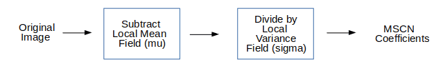
We have performed the metric on 4 types of distortions. Here is the final quality score, for each distortion:
| Original Image | JPEG2K Compression | Heavy Compression | Gaussian Noise | Median Blur |
|---|---|---|---|---|
 |  |  |  |  |
| 26.8286 | 30.7417 | 33.0692 | 79.8751 | 72.7044 |