Image Matting with state-of-the-art Method "F, B, Alpha Matting"

The foreground is the part of a view or picture, that is nearest to you when you look at it (Oxford dictionary). We, humans, are usually good at distinguishing foreground objects on images from the background. As computer vision algorithms became better and better at solving visual tasks it’s only natural we want to offload the foreground separation task to machines.

The problem of foreground-background separation is also called image matting and it arises in a wide spectrum of image-processing tasks. You can meet such algorithms in:

Film production sphere. Green-screens there are used to make a life of filmmakers easier allowing almost automatic foreground segmentation;
Video-conferencing apps. Some modern apps for web-conferencing (for example, Zoom) let users remove background from their web-cam image and replace it with something else;
Photo editing. The major application of image matting.

We know that foreground can be separated by applying semantic segmentation algorithms (like we did in one of the previous posts). Does this mean that the problem is virtually solved? Not exactly. The devil is always in details and in our case quite literally. The main difference between semantic segmentation and image matting is that in the latter we want our output to be extremely precise and continuous. Per-pixel labels identifying whether each particular pixel belongs to the foreground or background are no longer good enough for us since for a lot of natural objects like hair or fur the answer would be something in between. Most of the semantic segmentation algorithms are trained without making any emphasis on edges being that precise, so these models cannot give us the desired result. We need some special solution for our case, thus image matting.

We will return to the more formal problem definition later. Now let’s hop straight into the demo of the SOTA image matting algorithm to see how it works. We are grateful to the authors of the “F, B, Alpha Matting” article for providing the inference code which was used in our demo.

Demonstration

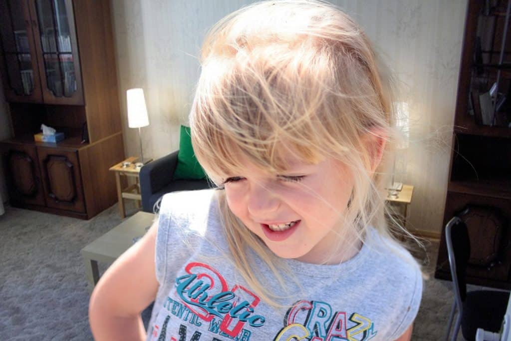
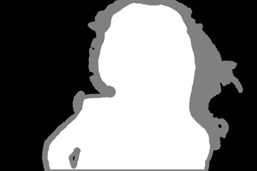
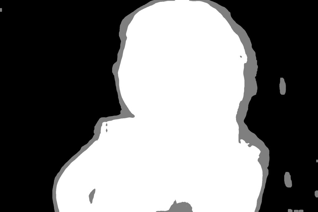
Let’s launch FBA Matting approach on real-life images. To apply FBA Matting algorithm we first need to generate a trimap (we’ll cover what it is later). In our demo, we’ll use a pre-trained DeepLabV3 to generate a segmentation mask with probabilities of each pixel belonging to a foreground class. After that we’ll use a number of dilation operations to mark border pixels and pixels with low foreground probability as unknown. Unfortunately, such an approach may lead to imprecise matting. You can see the difference between a labeled and a generated trimap below.

We’ll discuss the code for trimap generation in the following parts. Overall, our inference of FBA Matting consists of the next steps:

Produce segmentation of a person with DeepLabV3;
Apply dilation to get a trimap;
Use the generated trimap to predict the result with FBA Matting.

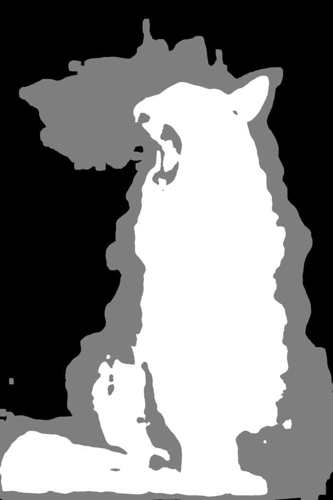
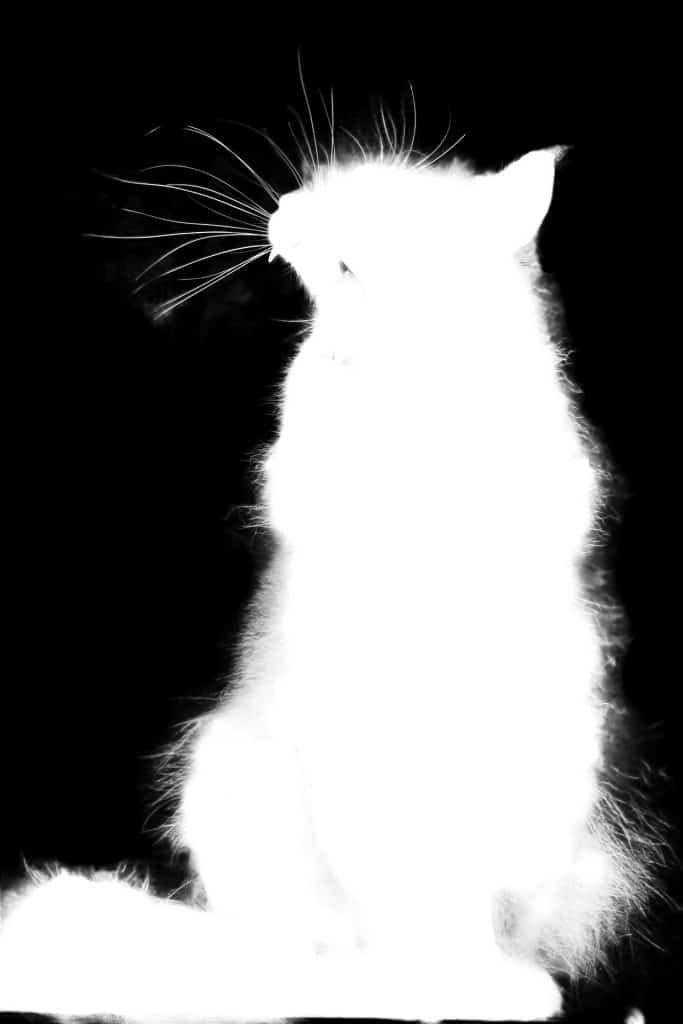
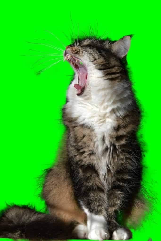
Here are the results of applying such an approach to the image of a cat can:

You can try it by yourself. Please, follow the instructions from the repository’s README.

Mathematical Formulation

Ok, now we saw that matting can generate pretty good results, but how does it work? Mathematically the issue is formulated as Compositing Equation:

$C_i=\alpha_iF_i+(1-\alpha_i)B_i$

If $\alpha_i$ equals 1 for pixel $i$ , then it’s a pure foreground pixel.

Solving the Compositing Equation is an ill-posed issue as we’ve only 3 equations for 7 unknowns. In the past few years several deep-learning-based methods have boosted the state-of-the-art in the image matting field. There are a lot of successful approaches such as Deep Image Matting,
IndexNet Matting, GCA Matting, to name but a few. The current state-of-the-art is F, B, Alpha Matting and today we are going to discuss it. But before that we need to figure out what a trimap is.

Trimap problem

We need to remember that the main focus of the matting problem is a very precise separation of the foreground from the background. Thus matting doesn’t actually care much about what type of an object is depicted on the image. This problem is decoupled from the actual semantic segmentation and because of that a lot of matting algorithms require segmentation
mask – or timap – as an input. Basically, the trimap is a rough segmentation of an image into three region types: certain foreground, unknown, certain background.

The trimap is usually concatenated with the corresponding image and then this 4-channel concatenation is used as an input for the model. However, this requirement imposes severe restrictions on the model usage. One should somehow generate the trimap from the image beforehand. It’s often expected to have some nice manually generated trimaps in order to run a matting algorithm on. Luckily, some authors suggest using a segmentation
network to predict the trimap from the source image – just what we did in our demo. We generate trimap using a segmentation mask, created by pre-trained DeepLabV3 as follows:

Download Code

Before we go over the explanation, you can download code from our GitHub repo:

Download Code To easily follow along this tutorial, please download code by clicking on the button below. It's FREE!

Click here to download the source code to this post

def trimap(probs, size, conf_threshold):
   """
   This function creates a trimap based on simple dilation algorithm
   Inputs [3]: an image with probabilities of each pixel being the foreground, size of dilation kernel,
   foreground confidence threshold
   Output    : a trimap
   """
   mask = (probs > 0.05).astype(np.uint8) * 255

   pixels = 2 * size + 1
   kernel = np.ones((pixels, pixels), np.uint8)

   dilation = cv2.dilate(mask, kernel, iterations=1)

   remake = np.zeros_like(mask)
   remake[dilation == 255] = 127  # Set every pixel within dilated region as probably foreground.
   remake[probs > conf_threshold] = 255  # Set every pixel with large enough probability as definitely foreground.

   return remake

F, B, Alpha Matting approach

The proposed method uses an encoder-decoder with U-Net style architecture. However, the most of previous approaches predict only alpha-matte while authors also predict $F$ and $B$ directly from this single encoder-decoder. In other words, model gives 7-channel output (1 for $\alpha$ , 3 for $F$ and 3 for $B$ ). Let’s now cover some tips and tricks the authors found particularly useful.

The encoder architecture is ResNet-50 with some modifications:

Three channels are used for an RGB image and the others are used for a trimap which in its turn is encoded with Gaussian blurs of the definite foreground and background masks at three different scales. Such encoding is the main difference from the previous approaches, as their authors usually encode the trimap as a single channel with values 1 for $F$ , 0.5 for unknown and 0 for $B$ .
The strides from layer3 and layer4 were removed and the dilations in these layers were increased to 2 and 4 respectively. The idea was to prevent lowering a feature map’s spatial resolution and process the information at the highest scales possible. Here is the encoder implementation:

class ResnetDilatedBN(nn.Module):
    def __init__(self, orig_resnet, dilate_scale=8):
        super(ResnetDilatedBN, self).__init__()
        from functools import partial

        if dilate_scale == 8:
            orig_resnet.layer3.apply(partial(self._nostride_dilate, dilate=2))
            orig_resnet.layer4.apply(partial(self._nostride_dilate, dilate=4))
        elif dilate_scale == 16:
            orig_resnet.layer4.apply(partial(self._nostride_dilate, dilate=2))

        # take pretrained resnet, except AvgPool and FC
        self.conv1 = orig_resnet.conv1
        self.bn1 = orig_resnet.bn1
        self.relu1 = orig_resnet.relu1
        self.conv2 = orig_resnet.conv2
        self.bn2 = orig_resnet.bn2
        self.relu2 = orig_resnet.relu2
        self.conv3 = orig_resnet.conv3
        self.bn3 = orig_resnet.bn3
        self.relu3 = orig_resnet.relu3
        self.maxpool = orig_resnet.maxpool
        self.layer1 = orig_resnet.layer1
        self.layer2 = orig_resnet.layer2
        self.layer3 = orig_resnet.layer3
        self.layer4 = orig_resnet.layer4

    def _nostride_dilate(self, m, dilate):
        classname = m.__class__.__name__
        if classname.find("Conv") != -1:
            # the convolution with stride
            if m.stride == (2, 2):
                m.stride = (1, 1)
                if m.kernel_size == (3, 3):
                    m.dilation = (dilate // 2, dilate // 2)
                    m.padding = (dilate // 2, dilate // 2)
            # other convolutions
            else:
                if m.kernel_size == (3, 3):
                    m.dilation = (dilate, dilate)
                    m.padding = (dilate, dilate)

Let’s discuss the input trimap generation process. First of all, we read the trimap as a gray-scale image and convert it into numpy array with shapes (H, W, 2) with the first channel for $F$ and the second for $B$ .

def read_trimap(name):
    trimap_im = cv2.imread(name, 0) / 255.0
    h, w = trimap_im.shape
    trimap = np.zeros((h, w, 2))
    trimap[trimap_im == 1, 1] = 1
    trimap[trimap_im == 0, 0] = 1
    return trimap

Then we scale the image and the trimap’s shapes so they are divisible by 8.

def scale_input(x: np.ndarray, scale: float, scale_type) -> np.ndarray:
    """ Scales inputs to multiple of 8. """
    h, w = x.shape[:2]
    h1 = int(np.ceil(scale * h / 8) * 8)
    w1 = int(np.ceil(scale * w / 8) * 8)
    x_scale = cv2.resize(x, (w1, h1), interpolation=scale_type)
    return x_scale

After that the trimap is transformed into a 6-channel form.

def dt(a):
    return cv2.distanceTransform((a * 255).astype(np.uint8), cv2.DIST_L2, 0)

def trimap_transform(trimap):
    h, w = trimap.shape[0], trimap.shape[1]

    clicks = np.zeros((h, w, 6))
    for k in range(2):
        if np.count_nonzero(trimap[:, :, k]) > 0:
            dt_mask = -dt(1 - trimap[:, :, k]) ** 2
            L = 320
            clicks[:, :, 3 * k] = np.exp(dt_mask / (2 * ((0.02 * L) ** 2)))
            clicks[:, :, 3 * k + 1] = np.exp(dt_mask / (2 * ((0.08 * L) ** 2)))
            clicks[:, :, 3 * k + 2] = np.exp(dt_mask / (2 * ((0.16 * L) ** 2)))

    return clicks

Then, a Pyramid Pooling layer is applied to the encoder features and the result is passed into the decoder with seven convolutional layers, three bilinear upsampling layers, and skip connections.

The Output contains 7 channels for $\alpha$ , $F$ , $B$ . The authors claim that clamping
the values of $\alpha$ between 0 and 1 with a hardtanh activation improves performance over using a sigmoid. The $F$ and $B$ logits are activated using the sigmoid.

Batch Normalization and Group Normalization

fter a number of experiments, the authors claimed that, quite counter-intuitively, the best results are achieved with a batch size equal to 1. However, it is impossible to use it as the original ResNet-50 has Batch Normalization layers which require batches with sizes larger than one. To overcome the issue, they suggest to use Group Normalization (32 channels per group) with Weight Standardization instead.

def norm(dim, bn=False):
    if bn is False:
        return nn.GroupNorm(32, dim)
    else:
        return nn.BatchNorm2d(dim)

A bouquet of Loss Functions

In most of the previous works a quite straight-forward loss politics have been used. For instance, in Deep Image Matting the final loss was formulated as a combination of an alpha-prediction loss:

$\mathcal{L}_{\alpha}^{i} = \sqrt{(\alpha_p^i - \alpha_g^i)^2 + \epsilon^2}, \alpha_p^i, \alpha_g^i \in [0, 1].$

and a compositional loss:

$\mathcal{L}_{c}^{i} = \sqrt{(c_p^i-c_g^i)^2 + \epsilon^2}.$

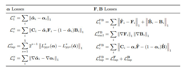
In “F, B, Alpha Matting” authors used a linear combination of eight different loss functions:

where $\mathcal{L}_1^\alpha$ is $\mathcal{L}_1$ loss on alpha, $\mathcal{L}_c^\alpha$ is the composition loss, $\mathcal{L}_g^\alpha$ is the gradient loss, and $\mathcal{L}_{lap}^\alpha$ is the Laplacian pyramid loss which is computed over multiple scales $s$ of the Laplacian pyramid $\mathcal{L}_{pyr}^s$ . For the $F$ and $B$ the
same losses were used as shown in the figure above.

The final loss was formulated as follows:

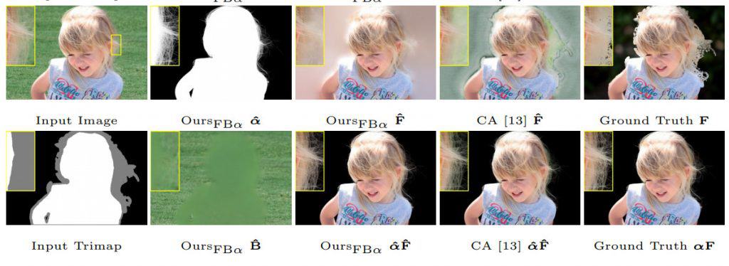
$\mathcal{L}_{FB\alpha} = \mathcal{L}_1^\alpha + \mathcal{L}_c^\alpha + \mathcal{L}_g^\alpha + \mathcal{L}_{lap}^\alpha + 0.25(\mathcal{L}_1^{FB} + \mathcal{L}_{lap}^{FB} + \mathcal{L}_{excl}^{FB}+ \mathcal{L}_{c}^{FB})$

As mentioned in the paper, it’s not enough to calculate the loss depending on absolute values of $\alpha$ only as these errors are not clearly visible. For example, errors in the reproduction of the hair strands shapes are more noticeable than slight errors in the overall opacity level. In Fig.2 you can see
that low $L_1$ doesn’t guarantee visually attractive predictions. That is why taking gradients in notice is quite important and it’s a reason to use gradient related losses such as $\mathcal{L}_g^\alpha$ and $\mathcal{L}_{lap}^\alpha$ .

visual-errors — **Fig.4:** Predictions with measured Sum of Absolute Difference

Fusion Strategy

One can see a problem with all those losses. Since the predictions for $\alpha$ , $F$ and $B$ produced by the model are decoupled, the relationship from the Compositing Equation is not performed. To deal with it, the authors proposed a fusion module based on the maximum likelihood estimate of $p(\alpha, F, B | \hat{\alpha}, \hat{F}, \hat{B})$ . They assumed the independence of the used errors and ignored any spatial dependence between pixels. It allowed them to build the likelihood model like this:

They also ssumed Gaussian distribution for the errors:

At last, they simplified the model by ignoring the gradient and Laplacian losses and replaced $\mathcal{L}_1$ with $\mathcal{L}_2$ Starting from, $\hat{F}^{(0)} = \hat{F}, \hat{B}^{(0)} = \hat{B}, \hat{\alpha}^{(0)} = \hat{\alpha}$ they used the following scheme:

The best results were achieved with $\sigma^2_C, \sigma^2_F, \sigma^2_B = 1, \sigma^2_\alpha=10.$

Overall, the fusion module helps to fuse all 3 predictions with respect to the Composing Equation.

Fusion module implementation:

def fba_fusion(alpha, img, F, B):
    F = alpha * img + (1 - alpha ** 2) * F - alpha * (1 - alpha) * B
    B = (1 - alpha) * img + (2 * alpha - alpha ** 2) * B - alpha * (1 - alpha) * F

    F = torch.clamp(F, 0, 1)
    B = torch.clamp(B, 0, 1)
    la = 0.1
    alpha = (alpha * la + torch.sum((img - B) * (F - B), 1, keepdim=True)) / (
        torch.sum((F - B) * (F - B), 1, keepdim=True) + la
    )
    alpha = torch.clamp(alpha, 0, 1)
    return alpha, F, B

Results

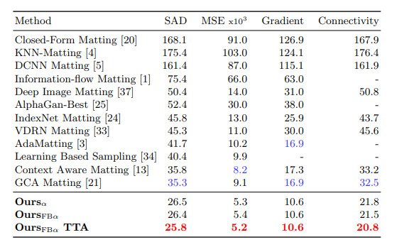
In Fig.3 and Fig.4 you can find results of the proposed method compared to the existing ones. TTA stands for test time augmentations, authors used a combination of rotation, flipping and scaling.

matting-results — **Fig.6:** Visualization of the results. CA stands for Context Aware Matting.

Conclusion

In our today’s post, we’ve discussed the challenging matting problem, tried the SOTA algorithm on our images and took a deeper look at how this algorithm works. We’ve tried to get around the requirement of manually generated trimap using a semantic segmentation network. It may be not a universal solution but it still produces decent results, especially if
one is ready to play with the parameters.