
GraphRAG integrates structured Knowledge Graphs (KGs) with semantic chunks (vectors), it enables LLMs to reason over multi-hop connections for complex queries and connect the dots between different sources offering holistic perspective.
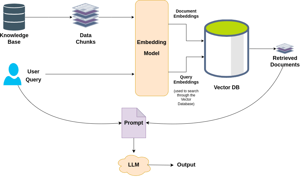
Retrieval Augmented Generation (RAG) has become the go-to approach for using LLM in real world, enterprise grade applications. By augmenting external knowledge sources, users can query over private corpora that weren’t part of model’s pre-training data. Traditional vector-based RAG approaches rely solely on semantic similarity. While they perform well for basic tasks, they often struggle with scalability, due to inefficacies such as flat data representation and lack of global context over the entire data corpus.
Let’s say you have a query seeking insights into how Medication A prescribed in Patient Record 1 influences the outcome of Condition B in Patient Record 2? Information like this may not be explicitly mentioned in the records, rather an LLM must infer the relationship by traversing chunks from both documents, to deduce the inter-dependencies and generate a meaningful response. Now, scale this requirement to medical institutions or health care companies handling hundreds of millions of patient records and notes. In complex scenarios like these, standard RAG will fall apart.

This is where GraphRAG (Graph + RAG) shines. Experimental studies and real world use cases have proven, GraphRAG offers more helpful and reliable responses than vector-only RAG. It’s a pivotal project from Microsoft, addressing the shortcomings of traditional RAG.
Synopsis of main topics that we will be covering are:
- Insights from original GraphRAG paper
- Fast GraphRAG, a faster and cost effective Approach
- Code Walkthrough of Fast GraphRAG Demo with Ollama
- Medical Document Analysis with Fast GraphRAG and Neo4j
“We’ve seen that a graph-based RAG approach is really efficient at helping self-orchestrating agentic AI get good at making the same kind of decisions a human would.”
– May Habib, CEO of Writer.com
- Limitations of Traditional RAGs
- Understanding Microsoft GraphRAG
- Key Features of GraphRAG
- Vector RAG vs GraphRAG
- Microsoft GraphRAG Workflow
- Benchmarks and Evaluation Metrics
- Shortcomings of Microsoft GraphRAG
- GraphRAG Alternatives and Improvements
- Fast GraphRAG
- Code Walkthrough: Medical Doc Analysis
- GraphML Data Visualization in Neo4j
- Limitations of Fast GraphRAG
- Conclusion
- References
This is the fourth article in our series of blogs on RAG.
- RAG with LLMs
- Multimodal RAG with ColPali and Gemini
- LightRAG: Legal Doc Analysis
- AgenticAI: A Comprehensive Introduction
Limitations of Traditional RAGs
- Lack of explainability: Since text chunks are represented as numerical vectors, it becomes difficult to accurately cite or trace the source of retrieved information leading to lack of transparency and verifiable grounding sources.
- Local Window: Standard RAG operates at a limited chunk-level context, therefore they fail to capture global context to incorporate relevant information from other parts of the corpus, resulting in an incomplete response.
- Scalability Issues: When working with large scale corpus especially in the medical and legal domain, semantic similarity alone may not always retrieve the most relevant chunks, producing suboptimal responses.
- Loss of Structural relationships: Baseline RAG approaches disregards the hierarchical structures and relationships between different levels of chunked information.
Understanding Microsoft GraphRAG
GraphRAG addresses these challenges by indexing information in a structured graph network called Knowledge Graphs (Ontology + Data).

— Knowledge Graphs —
Are you hearing the term for the very first time? Surprisingly, you’re already using this technology in your daily life. Google search, which handles billions of queries per day, internally uses Knowledge Graphs to show us the most relevant and optimal search results. Similarly, Facebook utilizes KGs to recommend friends and connections.
In the Pre-GenerativeAI Era, KGs were created using statistical or NLP techniques. However, GraphRAG scales efficiently by augmenting LLMs for extracting entities, claims and relationships along with their descriptions. In a KG, entities are represented as nodes and interlinked by edges that encode their relationships.
By spanning the broader scope of KG, GraphRAG can handle complex queries that are specifically targeted at global-level through Query Focussed Summarization (QFS).
The true advantage of KG lies in their ability to connect information from multiple sources, offering novel perspectives that may not be immediately apparent when analyzing isolated chunks of data. GraphRAG has proven to boost the retrieved accuracy and enables the LLM to reason over multi-hop nodes in the KG enabling reliable response.

For example:
Nodes :
| ENTITY TYPE | Entities |
| Disease | Diabetes, Hypertension, Pneumonia |
| Symptoms | Fatigue, High Blood Pressure, Cough |
| Medications | Metformin, Lisinopril, Azithromycin |
| Patient | Chris, Henry, Martha |
Edges:
| Source Entity | Relation | Target Entity |
| Chris | diagnosed_with | Diabetes |
| Metformin | prescribed_for | Diabetes |
| High Blood Pressure | leads_to | Heart Disease |
| Fatigue | symptom_of | Pneumonia |
Knowledge Graph: Use Cases
- Linkedin Custom Service QA
- Precina Health – Type 2 Diabetes
- Navigating Research Papers: Connected Papers
- Document Navigation
- SEO Assistants
- Graph Search Engine
Key Features of GraphRAG
- GraphRAG maintains multiple levels of hierarchical communities at different granularities, preserving both local and global information to generate actionable insights.
- By keeping the structures and relationships intact, GraphRAG ensures source traceability down to node level. This allows users to identify which sources contributed to the overall response, providing grounded citations that help to circumvent hallucinations.
- Unlike baseline RAG, which retrieves only a few
top_ksemantically similar chunks, offering a narrow or tunneled context to the LLM — GraphRAG aggregates information from multiple fragmented sources. This enables reasoning over multifaceted factors, generating a well-diversified answer while reducing any bias that arises from relying on only one source.
- During retrieval, GraphRAG disregards irrelevant information focusing solely on meaningful nodes and their connections for high-quality and coherent responses.
Vector RAG vs GraphRAG

| Feature | Traditional RAG | GraphRAG |
| Data Representation | Flat Vectors | Knowledge Graph |
| Query Scope | Local context | Global Reasoning |
| Scalability | Low | High |
| Citation Transparency | Low | High (Traceable sources) |
| Response Coherence | Fragmented | Relevant and Context-Rich |
Microsoft GraphRAG Workflow
We initially index our source documents and build the graph index followed by the querying phase.

Indexing Phase
It involves a two stage indexing process,
— STAGE 1: Generate Knowledge Graph —
Step 1: Segment Documents into Chunks
- Large corpora of text are split into manageable chunks to fit into the LLMs context window.
- Smaller chunks retain fine-grained information but it significantly increases the number of API calls, while larger chunks reduce cost but may miss critical information.
- Self reflection in prompts, improves response quality at a higher cost but ensures all the entities are extracted.
Step 2: Extract Entities and Relationships
- At this phase, the LLM is prompted to extract entities and relations within each chunk. Additionally LLM generates short descriptions about all entities and their relations.
- Each extracted entity is assigned a unique ID for traceability.
- Pronouns or ambiguous references in the chunks are resolved for clarity.
**-Goal-**
Given a text document that is potentially relevant to this activity and a list of entity types, identify all entities of those types from the text and all relationships among the identified entities.

-Steps-
1. Identify all entities. For each identified entity, extract the following information:
- entity_name: Name of the entity, capitalized
- entity_type: One of the following types: [{entity_types}]
- entity_description: Comprehensive description of the entity's
—-------------------------------------------------------------------
2. From the entities identified in step 1, identify all pairs of (source_entity, target_entity) that are *clearly related to each other.

For each pair of related entities, extract the following information:
- source_entity: name of the source entity, as identified in step 1
- target_entity: name of the target entity, as identified in step 1
- relationship_description: explanation as to why you think the source entity and the target entity are related to each other
- relationship_strength: a numeric score indicating strength of the relationship between the source entity and target entity
 # Entities:
{
  "nodes": [
    {
      "id": "n0",
      "entity_type": "PATIENT",
      "description": "A male patient aged 71 with several medical conditions",
      "source_id": "n0",
      "name": "71-YEAR-OLD GENTLEMEN"
    },
    {
      "id": "n1",
      "entity_type": "DIAGNOSIS",
      "description": "Condition treated with right leg angioplasty\nPeripheral vascular disease (PVD) is a circulatory condition characterized by narrowed or blocked arteries outside of the heart and brain, leading to reduced blood flow, particularly to limbs. Patients with PVD may have undergone procedures like angioplasty in affected areas to improve circulation. Treatment generally involves medications such as Plavix and aspirin, as well as surgical interventions based on individual assessments.",
      "source_id": "n1",
      "name": "PERIPHERAL VASCULAR DISEASE"
    },

. . .
# Relations
 "edges": [
    {
      "id": e0,
      "source": "n0",
      "target": "n1",
      "description": "The patient has a medical history of this condition",
    },
    {
      "id": e1,
      "source": "n0",
      "target": "n2",
      "description": "Chronic Obstructive Pulmonary Disease is part of his health profile",
    },
Step 3: Construct the Knowledge Graph (KG)
- The extracted entities and relationships are iteratively aggregated into a single unified KG.
- Multiple occurrences of the same element are merged to avoid duplicates.
— STAGE 2: Community Clustering —
Step 4: Graph Partitioning into Communities
- Once the KG is constructed, GraphRAG uses the Leiden community detection algorithm to partition the KG into semantically related clusters.
- The algorithm follows a hierarchical approach,where it recursively detects subcommunities until the leaf communities are reached, which can no longer be partitioned.
- It also ensures that each node belongs to only one community (mutually exclusive), and no node is left out from being assigned to a community.
- The size of the node is proportional to their importance or relevance degree.

Step 5: Community Summarization
The final step in the Indexing phase is, to aggregate various element summaries, where GraphRAG pipeline generates community summaries that capture the global structure and semantics of the dataset.
# **Goal**
Write a comprehensive report of a community, given a list of entities that belong to the community as well as their relationships and optional associated claims. The report will be used to inform decision-makers about information associated with the community and their potential impact. The content of this report includes an overview of the community's key entities, their legal compliance, technical capabilities, reputation, and noteworthy claims.
-----------------------------------------------------------------------------------------
# Report Structure
The report should include the following sections:

- TITLE: community's name that represents its key entities - title should be short but specific. When possible, include representative named entities in the title.
- SUMMARY: An executive summary of the community's overall structure, how its entities are related to each other, and significant information associated with its entities.
- IMPACT SEVERITY RATING: a float score between 0-10 that represents the severity of IMPACT posed by entities within the community.  IMPACT is the scored importance of a community.
- RATING EXPLANATION: Give a single sentence explanation of the IMPACT severity rating.
- DETAILED FINDINGS: A list of 5-10 key insights about the community. Each insight should have a short summary followed by multiple paragraphs of explanatory text grounded according to the grounding rules below. Be comprehensive.
With this, the LLM is capable of answering queries that are targeted at global overarching topics like “Who are the common people across the stories?”.
Here,
- Local : Leaf or lower level communities prioritize the most significant nodes and edges.
- Global: Higher-level communities aggregate multiple sub-communities, to ensure the most relevant information is retained while fitting within the LLM’s context window.
By this strategy, GraphRAG enables scalable and optimized analysis of large datasets targeting global context while maintaining fine granular details at node level.
This is why the paper is titled:
“From Local to Global: A GraphRAG Approach to Query-Focused Summarization”
Compared to source text summarizations, community summaries provides better responses for queries that are not targeted at leaf nodes.


Querying Phase
Query Focussed Summarization (QFS):
Key entities and relationships from user query are identified with similar patterns and correlations. These elements are then compared against community summaries. To make querying scalable and efficient, instead of analyzing the entire graph at once, only relevant community summaries are retrieved.
Map Reduce Approach:
- Map Phase: Each community report is processed parellely to generate multiple intermediate partial responses along with an
importance score(0 – 100), indicating how critical the point is in answering the given query.
- Reduce Phase: Then all the partial summaries are sorted in descending order based on the importance score, and high-scoring responses are combined to generate a Global answer.

To know more about the prompt used by the GraphRAG pipeline, at each intermediate steps, check out graphrag/prompts.
Benchmarks and Evaluation Metrics
To assess the effectiveness of GraphRAG for sensemaking-focused queries, traditional evaluation metrics such as RAGAS which calculates Faithfulness score, Answer and Context relevance aren’t right metrics. Since there isn’t no standardardized approach for this task, an LLM is used as a judge to compare the responses.
It evaluates the generated response bassed on:
- Comprehensiveness: How detailed and complete a response is, covering all the aspects of the query.
- Diversity: The richness of varied perspectives and insights offered.
- Empowerment: Determines whether a response aids in decision-making without any false assumptions.
- Directness: Assess how clear, concise and to the point the answer is.
GraphRAG outperforms naive RAG across comprehensiveness and diversity, however naive RAG scores better at generating directed answers.
Shortcomings of Microsoft GraphRAG
- Community based indexing and retrieval requires multiple LLM API calls, making the process slow, inefficient and extremely costly.
- There are no separate de-deplication steps carried out for repeated elements which results in a noisy graph index.
- In GraphRAG, to index a new data i.e. to upsert in existing KG, every time it will reconstruct the entire graph index, making it impractical for production use..
GraphRAG Alternatives and Improvements
GraphRAG, isn’t entirely new, early works of NebulaGraph, Langchain, LlamaIndex and Neo4j had their own version on graph-based RAG. Microsoft’s implementation was widely accepted as a compelling and the standard approach to GraphRAG. However, as we understood, it has its own limitations which led-to, follow-up works aimed at improving efficiency and accuracy.
Some notable variants of GraphRAG are:

To address the complexity associated with the original GraphRAG codebase, nano-graphragrag introduced a lighter and faster version. Unlike, the original graphrag which uses map-reduce approach to select the high scoring communities, nano selects only the top_k community, narrowing down the search results making it more efficient.
This lean design principle lead to multiple promising variants like LightRAG, MedGraphRAG, Fast GraphRAG etc which were built on top of it.
While working on a medical usecase for this article , we attempted to set up MedGraphRAG locally. However, adapting it for OpenAI compatible endpoints wasn’t straightforward.
Therefore, our primary objective of this article is to explore yet another scalable implementation from circlemind called Fast GraphRAG.
Fast GraphRAG
Benchmarks and experimental reports suggest, Fast GraphRAG performs 27x faster and 40% more accuracy in retrieval compared to other variants.
| Method | Accuracy (All Queries) | Accuracy (Multihop Only) – global | Insertion Time (minutes) |
| VectorDB | 0.42 | 0.23 | ~0.3 |
| LightRAG | 0.45 | 0.28 | ~25 |
| GraphRAG | 0.73 | 0.64 | ~40 |
| Fast GraphRAG | 0.93 | 0.90 | ~1.5 |
The graph construction economy principle recognizes that elaborate graph structures require significant computational resources to build. The investment must be justified by corresponding gains in retrieval performance, driving implementations toward economical approaches that maximize the performance-to-resource ratio.
At inference time, Fast GraphRAG uses a Page Rank algorithm similar to Google’s which determines the importance of an element within the KG. This efficient technique enables the system to retrieve and filter only the most relevant entities and their relations for generating high quality response.
Considering all these factors, you may need to evaluate Fast GraphRAG’s cost-to-performance ratio on your specific documents and entreprise to determine its viability as a suitable approach.
Now, that we have solid grasp of GraphRAG concepts, and it’s time to put theory to practice. Let’s go on a spree with experiments and test whether the benchmark claims hold true. The following code section, will guide you through project setup instructions. All the experiments were carried out on a RTX 3080 Ti GPU machine with 12 GB VRAM.

Code Walkthrough: Medical Doc Analysis with Fast GraphRAG
Fast GraphRAG, by default uses OpenAI SDK for API calls. This allows us to utilize any LLM providers of our choice which supports OpenAI Compatible API Endpoints by simply modifying the base_url.
—Ollama Local Setup : Phi4 14B—
We have tested several Ollama models under 14B class including Qwen, Deepseek, Gemma, Mistral-Nemo and Llama. However, a common issue we faced across these models was they were not able to generate response with proper structured output as expected by validators during summarize_entity_description stage in the Fast GraphRAG pipeline.
However this issue, didn’t occur with OpenAI or Gemini family of models in out testing, as they consistently produced structured outputs as expected without any flaws. The only model that worked successfully locally under 14B was Phi4 14B. While the exact reason is unclear, it could be attributed to the fact that the Phi models are primarily trained on a carefully curated dataset generated by GPT4.
If you have already installed ollama, run:
ollama pull phi4:14b.
The default 2K context length of Ollama’s configuration is very small, where a context length greater than 4K is more effective for searching global information. To address this, we will increase the context length to 6K by modifying the ModelFile. You can find more details about this from the ollama docs.
Open a new terminal and run:
ollama serve
to check the status of LLM and Embedding API calls, allowing us to debug and monitor the progress throughout the indexing phase and troubleshoot any issues.

As discussed earlier, in Fast GraphRAG all functions are asynchronous, enabling multiple concurrent API calls at a time. This works great with OpenAI or other providers who doesn’t impose rate limits per minute (RPM). However, when using Ollama, we encountered semaphore related issues.

To mitigate this, we can reduce the concurrent request limit as suggested in the README. In our case, we resolved this error by setting the CONCURRENT_TASK_LIMIT = 1, though this resulted in drop in indexing speed as we are missing out the perks of asynchronous parallel processing.
If you have found an better fix for this limitation, feel free to share your solution in issue#85 of the fastgraphrag repository.
# Modify slightly the source code

#FROM
#@throttle_async_func_call(max_concurrent=int(os.getenv("CONCURRENT_TASK_LIMIT", 8)), #stagger_time=0.001, waiting_time=10)
 #   async def send_message(. . .)

# TO
@throttle_async_func_call(
max_concurrent=int(os.getenv("CONCURRENT_TASK_LIMIT", 1)),
 stagger_time=0.001, waiting_time=0.1)
    async def send_message(. . .)

or
# in nano ~/.bashrc
# add
export CONCURRENT_TASK_LIMIT=1 # works without any error for ollama
Install Fast GraphRAG
!git clone https://github.com/circlemind-ai/fast-graphrag.git
%cd fast_graphrag
%poetry install

# or
!pip install fast-graphrag
Import Dependencies
import instructor  # To get **Structured outputs** for LLMs
import os
from fast_graphrag import GraphRAG, QueryParam
from fast_graphrag._llm import OpenAIEmbeddingService, OpenAILLMService
Dataset
For our experiments, we will be using the MIMIC (Medical Information Mart for Intensive Case) dataset, which is a publicly available dataset containing PII redacted electronic health records (EHR) from critical care patients, widely used for medical research. The original dataset contains 44,915 items, from that we will use from MIMIC-IV-ICU subset (mimic_ex) first 430 samples, with approximate around 650 words per .txt file.
# $ tree L 2 mimic_ex
mimic_ex_500/
├── report_0.txt
├── report_1.txt
├── . . .
├── report_499.txt
└── report_500.txt
Providing domain and entity types
In typical GraphRAG, defining the domain, example queries and entity types essentially guides the LLM during indexing phase to construct an effective knowledge graph.
DOMAIN: Ensures a focused extraction of medical entities from the documents.EXAMPLE_QUERIES: Few shot sample queries that conveys the user intent to the LLM.ENTITY_TYPES: Categorizes extracted entities in either one of the predefined typesworking_dir: Directory to save all the outputs
💡 Important Note: Ensure that the domain, sample queries, and entity types are adapted to match the specific document you are using for meaningful element extraction.
DOMAIN = "Analyze these clinical records and identify key medical entities. Focus on patient demographics, diagnoses, procedures, lab results, and outcomes."

EXAMPLE_QUERIES = [
    "What are the common risk factors for sepsis in ICU patients?",
    "How do trends in lab results correlate with patient outcomes in cases of acute kidney injury?",
    "Describe the sequence of interventions for patients undergoing major cardiac surgery.",
    "How do patient demographics and comorbidities influence treatment decisions in the ICU?",
    "What patterns of medication usage are observed among patients with chronic obstructive pulmonary disease (COPD)?"
]

ENTITY_TYPES = ["Patient", "Diagnosis", "Procedure", "Lab Test", "Medication", "Outcome", "Unknown"]

working_dir = "./WORKING_DIR/mimic_ex500/"
Configuring the Fast GraphRAG Pipeline
Next, we will initialize the GraphRAG(...) with a grag instance with specified configurations. To avoid unexpected data corrupt during indexing process, we can save the last n_checkpoints as backup, thanks to Fast GraphRAG’s state synchronization. By default ollama models runs on port 11434 and can be accessed as OpenAI compatible API endpoint by just setting the base_url as http://localhost:11434/v1
grag = GraphRAG(
    working_dir=working_dir,
    n_checkpoints=2, # to save backups (recommended)
    domain=DOMAIN,
    example_queries="\n".join(EXAMPLE_QUERIES),
    entity_types=ENTITY_TYPES,

    config=GraphRAG.Config(
        llm_service=OpenAILLMService(
            model="Phi4_6k",  # gemini-2.0-flash-exp
            # or https://generativelanguage.googleapis.com/v1beta/openai/
            base_url="http://localhost:11434/v1",  # Ollama
            api_key="ollama",  # or GEMINI_API_KEY
            mode=instructor.Mode.JSON,
            client="openai",   # default
        ),

        embedding_service=OpenAIEmbeddingService(
            model="mxbai-embed-large",  # mxbai-embed-large
            base_url="http://localhost:11434/v1",
            api_key="ollama",
            embedding_dim=1024,  # mxbai-embed-large - 1024 ; nomic-embed - 768
            client="openai"   # default
        ),
    ),
)

directory_path = "mimic_ex_430" # input dir to the dataset
Graph Indexing
The following utility function iterates through all the .txt files in the input directory and insert / upsert to construct the graph index. Fast GraphRAG indexing follows an incremental update algorithm which efficiently handles the duplicates by upserting the new files unlike Microsoft GraphRAG where the KG has to be reconstructed everytime.
def graph_index(directory_path):
    file_count = 0 # Keep track of processed files.

    for filename in os.listdir(directory_path):
        if filename.endswith('.txt'):
            file_path = os.path.join(directory_path, filename)
            with open(file_path, 'r') as file:
                content = file.read()

                # Convert list to string if needed
                    # If content follows a nested structure like {"text": "actual content"}
                if isinstance(content, list):
                    content = "\n".join(map(str, content))
                if isinstance(content, dict):
                    key_to_use = next(iter(content.keys()), None)
                    content = content[key_to_use] if key_to_use else str(content)

                else:
                    content = str(content)

                grag.insert(content)

            file_count += 1

            total_files = sum(1 for f in os.listdir(directory_path) if f.endswith(".txt"))
            print("******************** $$$$$$ *****************")
            print(f"Total Files Processed: -> {file_count} / {total_files}")
            print("******************** $$$$$$ *****************")
    return None

graph_index(directory_path)
Indexing all 430 items, took approximately 510 mins, (~ 8 hours, 30 mins), which is pretty reasonable and fast given the hardware constraints and the fact that it was processed locally with a 14B model.
Note: It’s is appropriate / fair to compare between different GraphRAG variants using OpenAI models as the API scales well without any errors.
📌 We have also tested Fast GraphRAG with free tier of Gemini Flash 2.0 from Google AI Studio on christmas carol by Dickens book. It took 110 API calls for a 32K words-document, making it a more budget-friendly option compared to GraphRAG.
All the output artifacts of the graph index will be saved under working_dir.
chunks_kv_data.pkl: Key-value mappings of text chunks for retrieval during querying.entities_hnsw_index_1024.bin: HNSW (Heirarchial Navigable Small World) index for efficient nearest-neighbor search. It stores vector embeddings of entities, enabling fast lookup and similarity search. Here1024indicates the embedding dimension.entities_hnsw_metadata.pkl: Metadata for entity embeddings, which includes entity IDs, type and description.graph_igraph_data.pklz: Compressed igraph-based representation of built KG, encompassing nodes and edges.map_e2r_blob_data.pkl: Mapping entity and relation interconnections.map_r2c_blob_data.pkl: Linking entities to text chunks for tracing source content.

Querying
Question 1: Targeted at Global
print(grag.query("Describe the sequence of interventions for patients undergoing major cardiac surgery?").response)
**********************************************
The sequence of interventions for the clinical scenario in post-aortic valve repair surgery with complications like respiratory issues, neurological impairment, and renal failure includes:

**Pre-surgery Preparation:**
- Evaluate and stabilize the patient.
- Manage existing conditions such as anemia and hypertension.
- Adjust or start medications like beta blockers (e.g., metoprolol) for blood pressure control and proton pump inhibitors (e.g., pantoprazole) to prevent gastrointestinal bleeding.

**Intraoperative Procedures:**
- Conduct aortic valve replacement or repair.
- Employ mechanical ventilation if necessary during and after surgery.
- Monitor cardiac function using pulmonary artery catheters for real-time hemodynamic data.

**Immediate Postoperative Care:**
- Continue invasive mechanical ventilation, especially in patients with respiratory issues or neurological impairments preoperatively.
- Closely monitor vital signs and organ functions, including renal and pulmonary systems.
- Administer medications for blood pressure management (e.g., pharmaceutical substances).

**Rehabilitation and Follow-up:**
- Perform swallow evaluation tests to ensure readiness for oral intake, followed by a diet progression to soft or clear liquids if necessary.
- Conduct physical and occupational therapy assessments to evaluate patient recovery progress.
- Schedule follow-up appointments for monitoring postoperative care including removal of surgical staples and further cardiac evaluations.

**Commonly Used Medications:**
- Anticoagulants (e.g., heparin) to prevent blood clots.
- Pain management medications like acetaminophen or hydromorphone.
- Diuretics such as furosemide for fluid balance and heart failure symptom management.

A multidisciplinary team including cardiologists, pulmonologists, and other specialists is often involved to address any comorbid conditions.
**********************************************

# o3-mini-high rated this response : 8/10.
Question 2: Targeted at Global
grag.query("How do patient demographics and comorbidities influence treatment decisions in the ICU?").response
**********************************************
Patient demographics and comorbidities significantly influence treatment decisions in the ICU, as evidenced by detailed hospital courses described in various scenarios.

1. **Demographics**: Specific ages or life stages, such as "on day of life 45" for a patient with unique medical conditions (metabolic issues), indicate tailored care plans sensitive to developmental stages.

2. **Comorbidities**:
   - A history like short gut syndrome and colectomy influences decisions about when and how to restart total parenteral nutrition (TPN). This reflects careful adaptation for chronic gastrointestinal needs and nutritional support in patients with limited absorptive capacities due to their past surgeries.
   - Comorbidity management, such as stabilizing hemodynamics through intravascular fluid resuscitation, pressors, blood products in hypovolemic shock cases or addressing complications post-lumbar artery bleed with transfusions of packed red blood cells, showcases ICU care adjustments based on acute exacerbations of chronic conditions.

3. **Interactions**: Decisions like replacing a PICC line with a Hickman catheter after infection shows proactive steps in avoiding repeat complications due to prior infections from central lines.
   - Balancing anticoagulants for patients historically having issues such as line clots, with adjustments like using lovenox instead of intravenous heparin, indicates treatment adaptations due to underlying heart or clotting disorders requiring long-term preventative strategies.

4. **Treatment Customization**: The management decisions, such as adjusting insulin administration for endocrine challenges even when insulin levels are normal, demonstrate personalized ICU therapy adapting for nuanced metabolic control in conditions like hypoglycemia of unknown origin.

These scenarios highlight that ICU treatment is deeply influenced by a patient’s demographic specifics and their spectrum of comorbidities, necessitating individualized care plans to address both acute and chronic health issues effectively.
**********************************************
# o3-mini-high rated this response : 8/10.
Question 3: Targeted at Global
print(grag.query("Provide indepth detail about in patients with both chronic obstructive pulmonary disease (COPD) and heart failure, how can lung function be improved?").response)
**********************************************
To optimize the treatment for patients with both COPD and heart failure,
it is crucial to manage fluids carefully using diuretics without causing respiratory issues.
This necessitates precise adjustments in medication dosages, closely monitoring fluid balance, and ensuring proper oxygenation levels.
Right heart catheterization can assist in measuring cardiac function and tailoring treatments for these patients.
The goal is to alleviate symptoms of both conditions while preventing exacerbations, which often involves using supplemental oxygen or bronchodilators as required.
**********************************************
# o3-mini-high rated this response : 8/10.
Question 4: Targeted at Local
print(grag.query("query ="Discuss about Hypocapnic and hypoxemic respiratory failure"?").response)
Hypocapnic Respiratory Failure and Hypoxemic Respiratory Failure are two distinct categories of respiratory failure, each characterized by different clinical features. Hypocapnic Respiratory Failure is associated with low blood levels of carbon dioxide (CO2), often caused by conditions like hyperventilation syndrome where excessive breathing leads to CO2 loss. Conversely, Hypoxemic Respiratory Failure involves reduced oxygenation of arterial blood and may occur in diseases such as chronic obstructive pulmonary disease (COPD) or pneumonia, where there is inadequate gas exchange at the alveoli. Accurate assessment and differentiation between these conditions are crucial for appropriate management and treatment.


In medical practice, both types may coexist or require different clinical interventions based on the specific underlying pathology.

**********************************************
# o3-mini-high rated this response : 6/10.

Fast GraphRAG also provides means to retrieve the reference or context of elements and chunks that being passed to the model by passing with_references = True as QueryParam.
# Querying with references
query = " Discuss about end-stage renal disease (ESRD)?"
answer = grag.query(query, QueryParam(with_references=True))

print(answer.response)  # ""
print(answer.context)  # {entities: [...], relations: [...], chunks: [...]}
GraphML Data Visualization in Neo4j
KGs contains complex interconnections and heirarchical structures, we can visualize and interact with them at node level by using Neo4j. For this, let’s start by saving the graph index in GraphML format.
os.makedirs("neo4j_graph", exist_ok=True)
grag.save_graphml(output_path="neo4j_graph/oxford_graph_chunk_entity_relation.graphml")
Preparing GraphML to JSON
#------------ neo4j_util.py ----------------------

import xml.etree.ElementTree as ET

NAMESPACE = "{http://graphml.graphdrawing.org/xmlns}"

def xml_to_json(xml_path):

    tree = ET.parse(xml_path)
    root = tree.getroot()

    # Find the <graph> element
    graph_elem = root.find(f".//{NAMESPACE}graph")

    nodes = []
    edges = []

    if graph_elem is None:
        return {"nodes": [], "edges": []}

    # --- Parse Nodes ---
    for node_elem in graph_elem.findall(f"{NAMESPACE}node"):
        node_id = node_elem.attrib.get("id")

        # Default structure
        node_data = {
            "id": node_id,
            "entity_type": None,
            "description": None,
            "source_id": node_id,  # Keep track of original ID if you want
            "name": None,
        }

        # Collect <data> children for this node
        for data_elem in node_elem.findall(f"{NAMESPACE}data"):
            key = data_elem.attrib.get("key", "")
            text_value = (data_elem.text or "").strip()

            if key == "v_type":
                node_data["entity_type"] = text_value
            elif key == "v_description":
                node_data["description"] = text_value
            elif key == "v_name":
                node_data["name"] = text_value

        nodes.append(node_data)

    # --- Parse Edges ---
    for edge_elem in graph_elem.findall(f"{NAMESPACE}edge"):
        edge_id = edge_elem.attrib.get("id")
        edge_source = edge_elem.attrib.get("source")
        edge_target = edge_elem.attrib.get("target")

        # If no explicit 'id' on the edge, generate one
        if not edge_id:
            edge_id = f"edge_{edge_source}_{edge_target}"

        edge_data = {
            "id": edge_id,
            "source": edge_source,
            "target": edge_target,
            "description": None,
            "source_id": edge_id,  # Keep the edge's own ID if you want
        }

        # Parse <data> elements for edges
        for data_elem in edge_elem.findall(f"{NAMESPACE}data"):
            key = data_elem.attrib.get("key", "")
            text_value = (data_elem.text or "").strip()

            if key == "e_description":
                edge_data["description"] = text_value
            # If you have more edge keys, parse them similarly:

        edges.append(edge_data)

    return {"nodes": nodes, "edges": edges}
Pushing to Neo4j AuraDB
Neo4j offers a free 1GB instance when you signup for the very first time. To avail, visit Neo4j AuraDB website and create a free instance. Personalize your credentials to push the KG from the converted json file to the instance DB. To get the INSTANCE_URI navigate to menu -> inspect and copy the Connection URI.

#------- neo4j_aura.py---------------

import os
import json
from neo4j_util import xml_to_json
from neo4j import GraphDatabase

# Constants
BATCH_SIZE_NODES = 500
BATCH_SIZE_EDGES = 100

# Neo4j connection credentials
NEO4J_URI = "INSTANCE_URI" #eg: neo4j+s://18847824.databases.neo4j.io
NEO4J_USERNAME = "neo4j"
NEO4J_PASSWORD = " " # Your instance Password


def convert_xml_to_json(xml_path, output_path):
    """Converts XML file to JSON and saves the output."""
    if not os.path.exists(xml_path):
        print(f"Error: File not found - {xml_path}")
        return None

    json_data = xml_to_json(xml_path)
    if json_data:
        with open(output_path, "w", encoding="utf-8") as f:
            json.dump(json_data, f, ensure_ascii=False, indent=2)
        print(f"JSON file created: {output_path}")
        return json_data
    else:
        print("Failed to create JSON data")
        return None


def process_in_batches(tx, query, data, batch_size):
    """Process data in batches and execute the given query."""
    for i in range(0, len(data), batch_size):
        batch = data[i : i + batch_size]
        tx.run(query, {"nodes": batch} if "nodes" in query else {"edges": batch})


def main():
    # Paths
    xml_file = "neo4j_graph/mimic430__graph_chunk_entity_relation.graphml"
    json_file = "neo4j_graph/json_mimic430__graph_chunk_entity_relation.json"

    # 1) Convert XML to JSON
    json_data = convert_xml_to_json(xml_file, json_file)
    if json_data is None:
        return

    # 2) Load nodes and edges from that JSON
    nodes = json_data.get("nodes", [])
    edges = json_data.get("edges", [])

    # 3) Define the Cypher queries

    # Create nodes (merges on id)
    create_nodes_query = """
    UNWIND $nodes AS node
    MERGE (e:Entity {id: node.id})
    SET e.entity_type = node.entity_type,
        e.description = node.description,
        e.source_id = node.source_id,
        e.displayName = node.id
    REMOVE e:Entity
    WITH e, node
    CALL apoc.create.addLabels(e, [node.id]) YIELD node AS labeledNode
    RETURN count(*)
    """

    # Create edges – uses edge.description as the relationship type
    # If edge.description is empty or None, default to 'IS'
    create_edges_query = """
    UNWIND $edges AS edge
    MATCH (source {id: edge.source})
    MATCH (target {id: edge.target})
    WITH source, target, edge,
         CASE
           WHEN edge.description IS NULL OR TRIM(edge.description) = '' THEN 'IS'
           ELSE TRIM(edge.description)
         END AS relType
    CALL apoc.create.relationship(
      source,
      relType,
      {
        description: edge.description,
        source_id: edge.source_id
      },
      target
    ) YIELD rel
    RETURN count(*)
    """

    # Optional: Set displayName and labels based on entity_type
    set_displayname_and_labels_query = """
    MATCH (n)
    SET n.displayName = n.id
    WITH n
    CALL apoc.create.setLabels(n, [n.entity_type]) YIELD node
    RETURN count(*)
    """

    # 4) Connect to Neo4j and run the queries in batches
    driver = GraphDatabase.driver(NEO4J_URI, auth=(NEO4J_USERNAME, NEO4J_PASSWORD))
    try:
        with driver.session() as session:
            # Insert nodes in batches
            session.execute_write(
                process_in_batches, create_nodes_query, nodes, BATCH_SIZE_NODES
            )

            # Insert edges in batches
            session.execute_write(
                process_in_batches, create_edges_query, edges, BATCH_SIZE_EDGES
            )

            # Set displayName and labels
            session.run(set_displayname_and_labels_query)

    except Exception as e:
        print(f"Error occurred: {e}")

    finally:
        driver.close()

if __name__ == "__main__":
    main()
Note: It create nodes in terms of unique ids (e.g., n01, n02 etc.) rather than meaningful entitiy names in english, it may feel abstract while visualizing the KG.
Limitations of Fast GraphRAG
- One of the main challenge we faced with Fast GraphRAG is that everything is asychronous and Pydantic-validated. For a beginner, this might be a nightmare when using local models.
- We observed that most 7B-class models struggle to generate structured responses and there is little to no documentation or community discussions about this. However, in LightRAG despite also been built on nano-graphrag, the well-documented pipeline for local LLMs, active community discussions directly answered by authors was much more pleasant experience.
- While Fast GraphRAG is faster than GraphRAG or LightRAG, it is still slower than vector only RAG. Graph-based RAG is ideal for large datasets requiring multi-hop queries, high stakes domains like medical accuracy cannot be compromised. But for simpler use cases, it’s recommended to use a naive vector-RAG.
Trivia
We faced challenges when indexing PDFs using pdf-plumber related to Pydantic validation errors. However it works with .txt files converted from PDFs using any online tools. We didn’t spend much time debugging this, but you can explore further.
Conclusion
GraphRAG enables monitoring behavioral patterns across different patients to deduce conclusive decisions with grounded edges and relations as citations. It empowers LLM to reason over complex, multi-hop queries and provide more accurate and context-rich responses. High stake domains where we can’t compromise on the accuracy and precision of retrieved information Graph-based RAG approaches are gamechanging offering holistic perspective that’s scalable and interpretable. Hybrid approaches combining knowledge graphs and vector embeddings performs better than naive RAG.
In this article, we went indepth discussing GraphRAG principles and concluded with Fast GraphRAG as an cost effective solution illustrated with a simple medical usecase. We recommend that before integrating GraphRAG directly in your pipeline, at first assess the requirements for your specific application within your enterprise and experiment extensively with various variants like LightRAG, Fast GraphRAG or HippoRAG. Based on response vibe checks and the retrieval quality choose suitable method that works best.
We hope you enjoyed the read! Do let us know, if you find it valuable via our social handles.
References
- Microsoft GraphRAG Paper
- FastGraphRAG Github
- HippoRAG
- MedGraphRAG Project
- LightRAG
- PageRank Algorithm


100K+ Learners
Join Free OpenCV Bootcamp3 Hours of Learning