In this post, we will learn how to perform image classification on arbitrary sized images without using the computationally expensive sliding window approach. This post is written for people who are familiar with image classification using Convolution Neural Networks.
Let’s first clear a big misconception about Convolutional Neural Networks (CNN).
Convolutional Neural Networks Do Not Need Fixed Sized Input
If you have ever used a CNN for image classification, you probably cropped and/or resized your input image to fit the input size the network requires.
While this practice is very common, there are a few limitations to using this approach.
- Loss of resolution : If you have a large image with dog that covers only small section of the image, then resizing the image will make the dog in the picture so small that the image will not be correctly classified.
- Non-square aspect ratio : Usually image classification networks are trained on square images. If the input image is not square, either a square region from the center is taken, or the width and height are resized using different scales to make the image square. In the first case, we may miss out of important features not in the center of the image, and in the second case the image information is distorted because of non-uniform scaling.
- Expensive sliding window approach : To mitigate the above problem, you may crop overlapping windows from the image, and perform image classification on each window. This is very expensive and as we will soon see entirely unnecessary.
The funny thing is that many people do not realize that a CNN can take any arbitrary sized image as input if we make minor modifications to the network. There is absolutely no retraining required!
In 2015, Dr. Yann Lecun, the head of Facebook AI and the inventor of CNNs, wrote in a short social media update to bring this misconception to light. If not not follow his quote below, don’t worry. We are here to explain in detail in this post.
In Convolutional Nets, there is no such thing as “fully-connected layers”. There are only convolution layers with 1×1 convolution kernels and a full connection table.
It’s a too-rarely-understood fact that ConvNets don’t need to have a fixed-size input. You can train them on inputs that happen to produce a single output vector (with no spatial extent), and then apply them to larger images. Instead of a single output vector, you then get a spatial map of output vectors. Each vector sees input windows at different locations on the input.
In that scenario, the “fully connected layers” really act as 1×1 convolutions.
Dr. Yann Lecun
How to Modify an Image Classification Architecture to Work on Arbitrary Sized Image
Almost all the classification architectures have a Fully-Connected (FC) layer at the end. ( Note: FC layer is called “Linear” Layer in PyTorch.)
The issue with the FC layers is that they expect input of the fixed size. If we change the spatial size of the input image, the inference will just fail.
So, we need to replace the FC layers with something else, but before we do that, let us understand why FC layers are used in the first place.
Why are Fully-Connected layers at Image Classification architectures?
Modern CNN architectures have several blocks of Convolutional Layers followed by a few FC layers in the end. This goes back to the very beginning of the Neural Networks research.
The basic idea is that blocks of Convolutional Layers extract semantic information from the image working as “smart” filters. To some extent, they preserve the spatial relations between the objects on the image.
However, to classify the object in the image we do not need this spatial information, so typically the output of the last convolutional layer is flattened into one long vector.
This long vector is the input for the FC layers that does not take into account the spatial information. The FC layers simply perform the weighted sum of the deep features across all the spatial locations in the image.
This structure works great – indeed, we can see it again and again in all the modern architectures, so, it is practice-proven.
However, because of the presence of FC layers, the network can only take fixed sized inputs.
So, we need to replace the FC layer with a different layer that does not require a fixed sized input. The good news is that we already have a layer that is not limited to the fixed size of its input – a Convolution layer!
Let’s see how to replace an FC layer with an equivalent Convolutional layer.
Fully-connected Layer to Convolution Layer Conversion
FC and convolution layer differ in the inputs they target – convolution layer focuses on local input regions, while the FC layer combines the features globally. However, FC and CONV layer both calculate dot products and therefore are fundamentally similar. Hence, we can convert one to another.
Let’s understand this by way of an example.
Let’s assume that there is an FC-layer is get’s its input from a Convolutional layer that outputs a 5x5x16 tensor. Let’s also assume the The FC layer output size is 120.
If we used an FC-layer, we would first flatten the 5x5x16 volume into a 400×1 ( i.e. 5x5x16 ) vector for the FC-layer.
However, we are going to use an equivalent convolution layer. For that we need to use a kernel of size 5x5x16. In CNNs, we the kernel depth (which is 16 in this case) is always the same as the the depth of the input, and usually the width and height are the same (5 in this case). So we can simply say the kernel size is 5 instead of saying it is 5x5x16.
The number of filters = 120 which is the same as the output we want.
As you can guess the stride = 1 and padding = 0.
How to modify ResNet-18 Architecture to work on Arbitrary Sized Image

ResNet-18 is a popular CNN architecture and PyTorch comes with pre-trained weights for ResNet-18.
The expected input size for the network is 224×224, but we are going to modify it to take in an arbitrary sized input.
Resnet-18 architecture starts with a Convolutional Layer. In PyTorch’s implementation, it is called conv1 (See code below).
This is followed by a pooling layer denoted by maxpool in the PyTorch implementation.
This in turn is followed by 4 Convolutional blocks shown using pink, purple, yellow, and orange in the figure. These blocks are named layer1, layer2, layer3, and layer4.
Each block contains 4 convolutional layers.
Finally, we have an average pooling layer denoted by avgpool in the code. The output of this layer is flattened and fed to the final fully connected layer denoted by fc.
The following code is copied from the resnet.py file and it is the implementation of Resnet in torchvision. You can compare it with the figure above.
# from the torchvision's implementation of ResNet

class ResNet:

    # ...
    self.conv1 = nn.Conv2d(3, self.inplanes, kernel_size=7, stride=2, padding=3,
                               bias=False)
        self.bn1 = norm_layer(self.inplanes)
        self.relu = nn.ReLU(inplace=True)
        self.maxpool = nn.MaxPool2d(kernel_size=3, stride=2, padding=1)
        self.layer1 = self._make_layer(block, 64, layers[0])
        self.layer2 = self._make_layer(block, 128, layers[1], stride=2, dilate = replace_stride_with_dilation[0])
        self.layer3 = self._make_layer(block, 256, layers[2], stride=2, dilate = replace_stride_with_dilation[1])
        self.layer4 = self._make_layer(block, 512, layers[3], stride=2, dilate = replace_stride_with_dilation[2])
        self.avgpool = nn.AdaptiveAvgPool2d((1, 1))
        self.fc = nn.Linear(512 * block.expansion, num_classes)

    # ...

    def _forward_impl(self, x):
        # See note [TorchScript super()]
        x = self.conv1(x)
        x = self.bn1(x)
        x = self.relu(x)
        x = self.maxpool(x)

        x = self.layer1(x)
        x = self.layer2(x)
        x = self.layer3(x)
        x = self.layer4(x)

        x = self.avgpool(x)
        x = torch.flatten(x, 1)
        x = self.fc(x)

        return x
We are going to create a new class FullyConvolutionalResnet18 by inheriting from the original torchvision ResNet class in torchvision.
The code is explained in the comments but please note two important points
- In PyTorch
AdaptiveAvgPool2dis applied before the fully connected layer. This is not part of the original ResNet architecture but simply an implementation detail.AdaptiveAvgPool2dcollapses the feature maps of any size to the predefined one. This allows torchvision ResNet implementation to take an image of any size as input. Many implementations do not have such an “adaptive” layer and use the pooling with the pre-defined window size. As a consequence FC layer will get the input of size it does not expect (e.g. torchvision 0.2 or earlier versions had this implementation). What’s worse, even with the adaptive average pooling applied, we have very different results with the different input image resolution. So, we have replacedAdaptiveAvgPool2dwithAvgPool2d. - We have converted the FC layer with a Convolutional layer by copying weights and biases.
Now, let’s go over the code while paying attention to the comments.
class FullyConvolutionalResnet18(models.ResNet):
    def __init__(self, num_classes=1000, pretrained=False, **kwargs):

        # Start with standard resnet18 defined here
        super().__init__(block = models.resnet.BasicBlock, layers = [2, 2, 2, 2], num_classes = num_classes, **kwargs)
        if pretrained:
            state_dict = load_state_dict_from_url( models.resnet.model_urls["resnet18"], progress=True)
            self.load_state_dict(state_dict)

        # Replace AdaptiveAvgPool2d with standard AvgPool2d
        self.avgpool = nn.AvgPool2d((7, 7))

        # Convert the original fc layer to a convolutional layer.
        self.last_conv = torch.nn.Conv2d( in_channels = self.fc.in_features, out_channels = num_classes, kernel_size = 1)
        self.last_conv.weight.data.copy_( self.fc.weight.data.view ( *self.fc.weight.data.shape, 1, 1))
        self.last_conv.bias.data.copy_ (self.fc.bias.data)

    # Reimplementing forward pass.
    def _forward_impl(self, x):
        # Standard forward for resnet18
        x = self.conv1(x)
        x = self.bn1(x)
        x = self.relu(x)
        x = self.maxpool(x)

        x = self.layer1(x)
        x = self.layer2(x)
        x = self.layer3(x)
        x = self.layer4(x)
        x = self.avgpool(x)

        # Notice, there is no forward pass
        # through the original fully connected layer.
        # Instead, we forward pass through the last conv layer
        x = self.last_conv(x)
        return x
Using Fully Convolutional ResNet-18 – Fully Convolutional Image Classification
Let’s see how to use this new version of ResNet-18 in our code.
1. Import Standard Libraries
import torch
import torch.nn as nn
from torchvision import models
from torch.hub import load_state_dict_from_url

from PIL import Image
import cv2
import numpy as np
from matplotlib import pyplot as plt
2. Read ImageNet class id to name mapping
if __name__ == "__main__":

    # Read ImageNet class id to name mapping
    with open('imagenet_classes.txt') as f:
        labels = [line.strip() for line in f.readlines()]
3. Read image and transform it to be ready to use with PyTorch.

    # Read image
    original_image = cv2.imread('camel.jpg')

    # Convert original image to RGB format
    image = cv2.cvtColor(original_image, cv2.COLOR_BGR2RGB)

    # Transform input image
    # 1. Convert to Tensor
    # 2. Subtract mean
    # 3. Divide by standard deviation

    transform = transforms.Compose([
                 transforms.ToTensor(), #Convert image to tensor.
                 transforms.Normalize(
                 mean=[0.485, 0.456, 0.406],   # Subtract mean
                 std=[0.229, 0.224, 0.225]     # Divide by standard deviation
                 )])

    image = transform(image)
    image = image.unsqueeze(0)
4. Load FullyConvolutionalResNet18 model with pre-trained weights.
    # Load modified resnet18 model with pretrained ImageNet weights
    model = FullyConvolutionalResnet18(pretrained=True).eval()
5. Perform Inference to Obtain Response Map
    with torch.no_grad():
        # Perform inference.
        # Instead of a 1x1000 vector, we will get a
        # 1x1000xnxm output ( i.e. a probabibility map
        # of size n x m for each 1000 class,
        # where n and m depend on the size of the image.)
        preds = model(image)
        preds = torch.softmax(preds, dim=1)

        print('Response map shape : ', preds.shape)

        # Find the class with the maximum score in the n x m output map
        pred, class_idx = torch.max(preds, dim=1)
        print(class_idx)

        row_max, row_idx = torch.max(pred, dim=1)
        col_max, col_idx = torch.max(row_max, dim=1)
        predicted_class = class_idx[0, row_idx[0, col_idx], col_idx]

        # Print top predicted class
        print('Predicted Class : ', labels[predicted_class], predicted_class)
When the above code is run, we receive the following output
Response map shape :  torch.Size([1, 1000, 3, 8])
tensor([[[977, 977, 977, 977, 977, 978, 354, 437],
         [978, 977, 980, 977, 858, 970, 354, 461],
         [977, 978, 977, 977, 977, 977, 354, 354]]])
Predicted Class :  Arabian camel, dromedary, Camelus dromedarius tensor([354])
In the original ResNet implementation, the output is vector of 1000 elements where each element of the vector correspond to the class probabilities of the 1000 classes of ImageNet.
In the fully convolutional version, we get a response map of size [1, 1000, n, m] where n and m depend on the size of the original image and the network itself.
In our example, when we forward pass an image of size 1920×725 through the network, we receive a response map of size [1, 1000, 3, 8].
The result can be interpreted as the inference performed on 3 x 8 = 24 locations on the image by obtained sliding window of size 224×224 ( the input image size for the original network ).
6. See the Response Map for the Predicted Class
Next, we find the response map for the predicted class and upsample it to fit the original image.
We threshold the response map to obtain the area of interest and find a bounding box around it.
        # Find the n x m score map for the predicted class
        score_map = preds[0, predicted_class, :, :].cpu().numpy()
        score_map = score_map[0]

        # Resize score map to the original image size
        score_map = cv2.resize(score_map, (original_image.shape[1], original_image.shape[0]))

        # Binarize score map
        _, score_map_for_contours = cv2.threshold(score_map, 0.25, 1, type=cv2.THRESH_BINARY)
        score_map_for_contours = score_map_for_contours.astype(np.uint8).copy()

        # Find the countour of the binary blob
        contours, _ = cv2.findContours(score_map_for_contours, mode=cv2.RETR_EXTERNAL, method=cv2.CHAIN_APPROX_SIMPLE)

        # Find bounding box around the object.
        rect = cv2.boundingRect(contours[0])
7. Display Results
The following code is used to display the results graphically. We use the response map to highlight the regions the show high likelihood of the predicted class.
        # Apply score map as a mask to original image
        score_map = score_map - np.min(score_map[:])
        score_map = score_map / np.max(score_map[:])

Next we multiply the response map with the original image and display the bounding box.
        score_map = cv2.cvtColor(score_map, cv2.COLOR_GRAY2BGR)
        masked_image = (original_image * score_map).astype(np.uint8)

        # Display bounding box
        cv2.rectangle(masked_image, rect[:2], (rect[0] + rect[2], rect[1] + rect[3]), (0, 0, 255), 2)

        # Display images
        cv2.imshow("Original Image", original_image)
        cv2.imshow("scaled_score_map", score_map)
        cv2.imshow("activations_and_bbox", masked_image)
        cv2.waitKey(0)
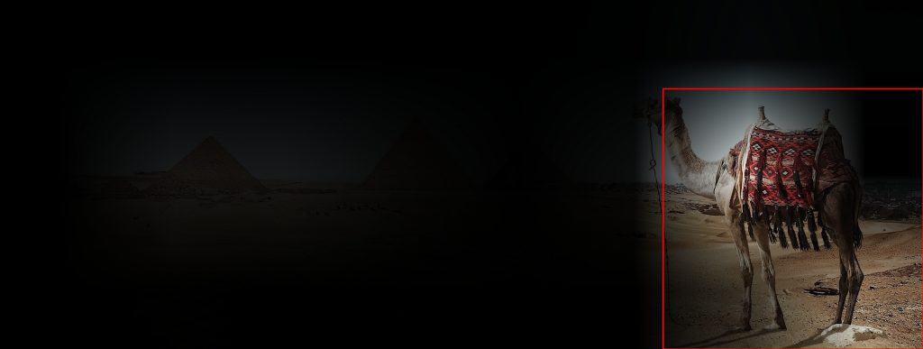
The result is shown below. Can you can see only the camel gets highlighted. The bounding box created by thresholding the response map captures the camel. In this sense, a fully convolutional image classifier acts like an object detector!








100K+ Learners
Join Free OpenCV Bootcamp3 Hours of Learning