The agricultural and food industry relies heavily on the crop lifecycle. But did you know leaf diseases are a significant threat to agriculture worldwide? They reduce crop yields and harm food security. Around 30% of crops are lost each year due to plant diseases, causing financial losses of over $40 billion. This problem becomes even more serious when we consider that over 821 million people have faced hunger in recent years. What if we could detect these diseases early, help our farmers, and boost the agricultural economy? Well finetuning SAM2 can help!
But how finetuning SAM2 can solve our problem that we are gonna explore now. In this article, we will finetune the segment anything model 2 (SAM2) to detect and segment out the diseased portion of the leaf. Let’s get started!
- What is Leaf Disease Segmentation?
- Why Fine-Tune SAM2 for This Task?
- Challenges of Finetuning SAM2 for Leaf Disease Segmentation
- Building the Leaf Segmentation Dataset
- Setting Up the Environment
- Imports and Setup
- Setting the Seed for Reproducibility
- Data Loading and Splitting
- Data Preprocessing and Visualization
- Building the SAM2 Model
- Training Configuration for Finetuning SAM2
- Training and Validation Loops
- Inference on Finetuned SAM2
- Quick Recap
- Conclusion
- References
What is Leaf Disease Segmentation?
Leaf disease segmentation is nothing but segmenting the damaged area of the leaves in the plant. But before we go into technicality, we need to understand what leaf disease actually is? Various pathogens, including fungi, bacteria, and viruses, can cause leaf diseases. Some prevalent leaf diseases include:
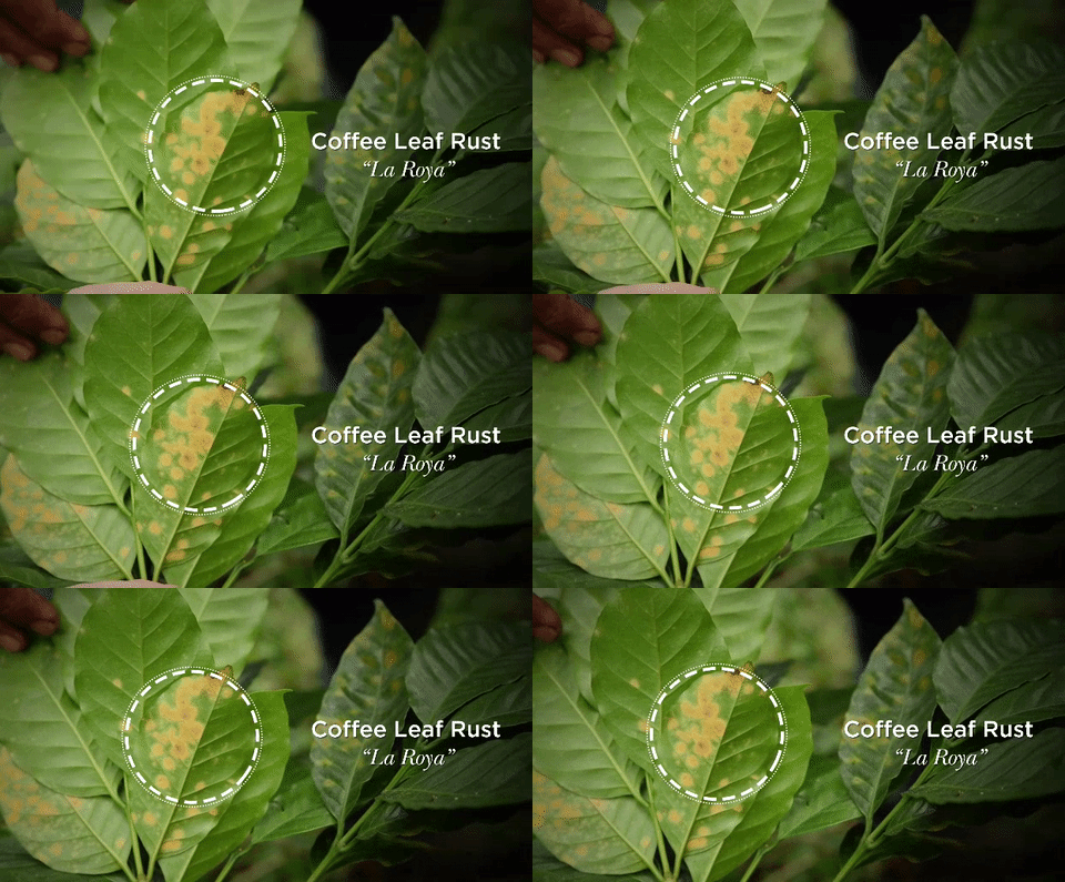
- Leaf Spot – Affects crops like rice, maize, and peanuts.
- Rust Diseases – Common in many crops, leading to significant yield reductions.
- Coffee Leaf Rust – Responsible for severe losses in coffee production in Central America.
The economic implications of these diseases are staggering. For instance, losses in key crops such as wheat (10-28%), rice (25-41%), and maize (20-41%) threaten global food supply chains. Moreover, diseases like Xylella fastidiosa have led to job losses in sectors such as olive oil production, further highlighting the socio-economic impact of plant diseases. Overall, reduced production affects the entire economy, from farmers to consumers, in terms of both money and food.
What if we could detect and segment diseased (or damaged) regions early using deep learning? This could provide significant benefits… Let’s think of several possible scenarios for finetuning SAM2:
- Preventative Action – Timely identification allows farmers to take action before the disease spreads to other parts of the plant or neighboring crops.
- Economic Savings – By preventing widespread infection, farmers can save on costs associated with crop loss and treatment.
- Food Security – With a growing global population, ensuring crop health is vital for maintaining food supply and preventing hunger.

But wait, implementing early detection systems not only prevents the infection but also leads to:
- Increased Crop Yields – By identifying and managing diseases early, farmers can maintain higher productivity yields.
- Reduced Chemical Use – Early intervention can minimize the reliance on pesticides and fungicides, promoting sustainable farming practices.
- Enhanced Quality of Produce – Healthier plants lead to better quality crops, which can fetch higher market prices.
Now, we have a better understanding of our problem statement. So, let’s proceed further with the solution.
Why Fine-Tune SAM2 for This Task?
As the article title suggests, the solution will be very simple: we will use SAM2 as our segmentation model and a leaf disease dataset to finetune the model. Now the question arises: Why specifically SAM2?

While robust segmentation models like U-Net, DeepLabV3, SegFormer, exists, what makes SAM2 stand out is:
SAM2 is trained on the SA-V dataset, one of the largest and most diverse video segmentation datasets. Due to its extensive pretraining, SAM2 can segment almost anything without fine-tuning (the best Zero-Shot Segmentation model so far.). Even if you have a really small dataset, you can still finetune SAM2 effectively, enabling high segmentation accuracy for domain-specific tasks.
It comes with a unique architecture where it provides promptable segmentation, meaning it can segment objects based on user-defined prompts like points, boxes, or masks. If you look at the architecture of SAM2:

It follows almost the same architecture as SAM, adding memory attention and a memory bank for video segmentation, making it unique. You can simply use your image or video, provide a prompt like points or bounding box coordinates (e.g., “segment the dog and football here”), and you can check out our detailed article about SAM2 to get a quick overview of the model.
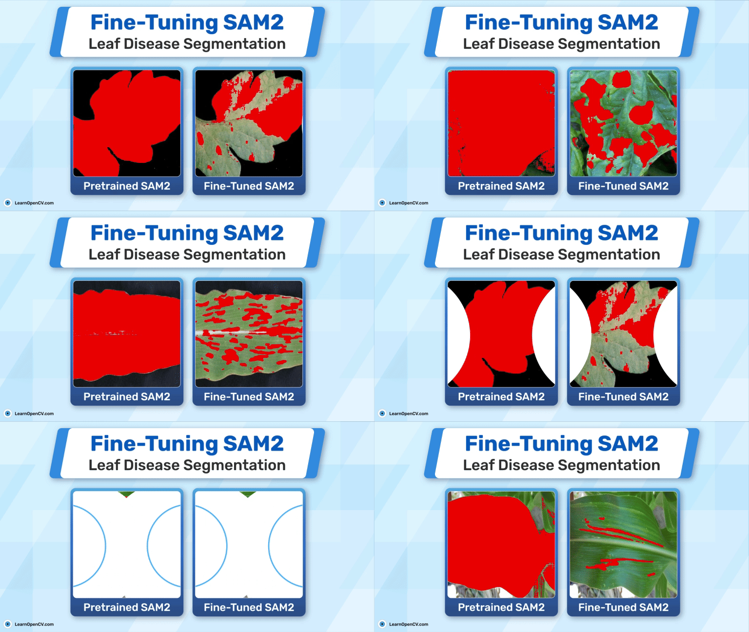
Also, we tried the pre trained SAM2 model on our test data to see if it could segment the diseased areas, you can see the results:
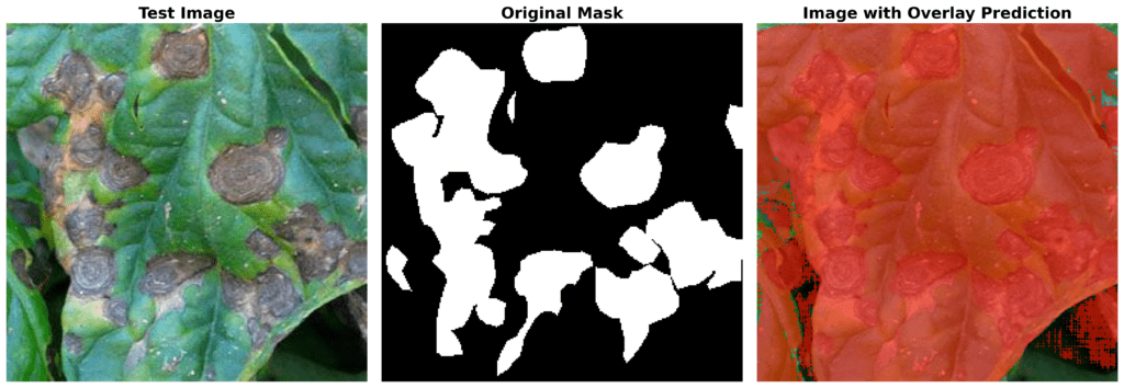
As you can see it’s not able to do that, and that’s not its fault. Our task is deeply domain-specific that even SAM2 alone can’t segment these diseased leaves accurately without fine-tuning.t. So, we have to fine-tune it to get the accurate results.
In this article, we will use SAM2 for image segmentation. We will cover video finetuning in one of our future articles. Let’s see the challenges we might face while finetuning SAM2 for Leaf Disease Segmentation.
New to segmentation? Check out our free TensorFlow Bootcamp to get started!
Challenges of Finetuning SAM2 for Leaf Disease Segmentation
The very first problem is the availability of data. There isn’t a significant amount of leaf disease segmentation data available on the internet. We are using the leaf disease segmentation dataset from Kaggle, which consists of 588 image-mask pairs. Now, you can understand why we chose SAM2. Given the limited amount of data available, SAM2 became the ideal choice for our problem.
Another challenge is fine-tuning SAM2. Unlike most segmentation models, SAM2 fine-tuning follows a different approach. After exploring various strategies, we found that using points as a prompt along with the binary mask works best for our case. We will explore this further in the training SAM2 code.
Last but not least, While SAM2 is highly efficient for segmentation, fine-tuning it requires significant computational power. The model is pre-trained on a large dataset and consists of transformer-based architectures, making it computationally intensive. If you don’t have access to high-end GPUs (A100, V100, or RTX 3090/4090), fine-tuning may take considerable time. Let’s see if we can train it on a laptop GPU like RTX 3070 Ti.
Enough theory—let’s dive into the code! Grab a coffee, sit with your laptop, and be ready to explore. This is where things get exciting!
Building the Leaf Segmentation Dataset
For finetuning SAM2, we will use the dataset from Kaggle, with a few modifications:
.
├── images
├── masks
└── train.csv
- Images – This folder contains 588 RGB images showcasing various types of leaf diseases.
- Masks – This folder holds 588 RGBA segmentation masks, where the diseased regions of the leaves are annotated.
- train.csv – A CSV file that maps each image to its corresponding segmentation mask, ensuring proper indexing for SAM2 training.
Let’s look at some of the training samples:
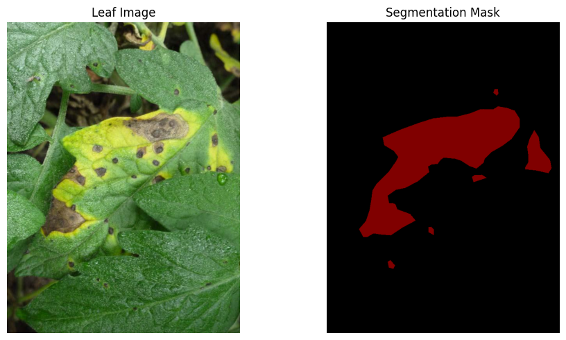
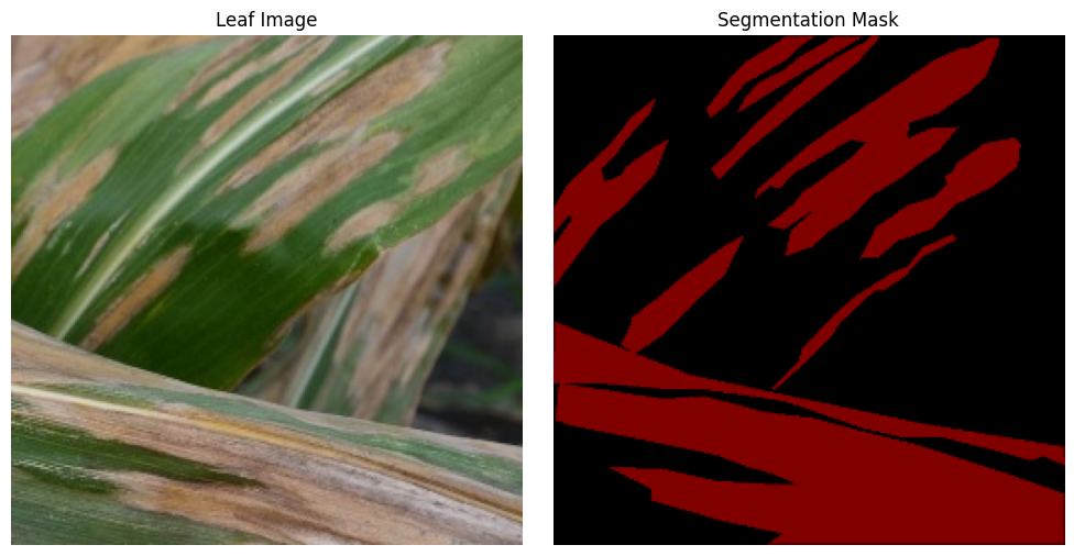

Let’s start setting up the environment for fine-tuning SAM2 now.
However, you need to preprocess the data. We will provide the necessary code for this. Click the Download Code button below and get started!
Setting Up the Environment for Finetuning SAM2
First, we will create a virtual environment in our workspace. We are using Miniconda here.
!conda create -n your_env python=3.9.0
!conda activate your_env
To begin the fine-tuning process, we need to install the SAM-2 library, which is essential for the Segment Anything Model (SAM2). This model is built to handle various segmentation tasks efficiently. The installation involves cloning the SAM-2 repository from GitHub and setting up the required dependencies.
!git clone https://github.com/facebookresearch/segment-anything-2
%cd /content/segment-anything-2
!pip install -q -e .
Now, we will download the dataset:
# get dataset from Kaggle
from google.colab import files
files.upload()  # This will prompt you to upload the kaggle.json file

!mkdir -p ~/.kaggle
!mv kaggle.json ~/.kaggle/
!chmod 600 ~/.kaggle/kaggle.json
!kaggle datasets download -d ankanghosh651/leaf-sengmentation-dataset-sam2-format
Let’s unzip it now:
!sudo apt-get install zip unzip
!unzip leaf-sengmentation-dataset-sam2-format.zip -d ./leaf-seg
We are done with the dataset download, Next, let’s download the SAM2 model weights:
!wget -O sam2_hiera_tiny.pt "https://dl.fbaipublicfiles.com/segment_anything_2/072824/sam2_hiera_tiny.pt"
!wget -O sam2_hiera_small.pt "https://dl.fbaipublicfiles.com/segment_anything_2/072824/sam2_hiera_small.pt"
!wget -O sam2_hiera_base_plus.pt "https://dl.fbaipublicfiles.com/segment_anything_2/072824/sam2_hiera_base_plus.pt"
!wget -O sam2_hiera_large.pt "https://dl.fbaipublicfiles.com/segment_anything_2/072824/sam2_hiera_large.pt"
We will use sam2_hiera_tiny.pt since we should be able to run it on a free-tier GPU or our local GPU.
Now, let’s move on to the main part and begin fine-tuning SAM2 for leaf disease segmentation.
Finetuning SAM2 – Imports and Setup
import os
import random
import pandas as pd
import cv2
import torch
import torch.nn.utils
import torch.nn.functional as F
import numpy as np
import matplotlib.pyplot as plt
import matplotlib.colors as mcolors
from sklearn.model_selection import train_test_split

from sam2.build_sam import build_sam2
from sam2.sam2_image_predictor import SAM2ImagePredictor
The custom modules build_sam2 and SAM2ImagePredictor are imported from the cloned SAM2, where build_sam2 sets up the network architecture with our chosen checkpoint, and SAM2ImagePredictor loads the model for further processing.
Setting the Seed for Reproducibility
def set_seeds():
    SEED_VALUE = 42
    random.seed(SEED_VALUE)
    np.random.seed(SEED_VALUE)
    torch.manual_seed(SEED_VALUE)
    if torch.cuda.is_available():
        torch.cuda.manual_seed(SEED_VALUE)
        torch.cuda.manual_seed_all(SEED_VALUE)
        torch.backends.cudnn.deterministic = True
        torch.backends.cudnn.benchmark = True

set_seeds()
For deterministic results and reproducibility, we will set a fixed seed value to ensure consistent runs across different runs. This is a very common strategy for Finetuning SAM2 or any other model.
Data Loading and Splitting
data_dir = "../leaf-seg/leaf-seg"
images_dir = os.path.join(data_dir, "images")
masks_dir = os.path.join(data_dir, "masks")

train_df = pd.read_csv(os.path.join(data_dir, "train.csv"))

train_df, test_df = train_test_split(train_df, test_size=0.2, random_state=42)

train_data = []
for index, row in train_df.iterrows():
   image_name = row['imageid']
   mask_name = row['maskid']
   train_data.append({
       "image": os.path.join(images_dir, image_name),
       "annotation": os.path.join(masks_dir, mask_name)
   })

test_data = []
for index, row in test_df.iterrows():
   image_name = row['imageid']
   mask_name = row['maskid']
   test_data.append({
       "image": os.path.join(images_dir, image_name),
       "annotation": os.path.join(masks_dir, mask_name)
   })
In this segment, we start by defining file paths to our dataset directories. The CSV file, train.csv, holds metadata pairing images (`imageid`) with their masks (`maskid`). We use train_test_split from scikit-learn to partition our data into training and testing sets, allocating 80% to training and 20% to validating. Each entry in train_data and test_data is a dictionary containing the file paths for the corresponding image and mask, enabling easy iteration during training and validation.
Data Preprocessing and Visualization
def read_batch(data, visualize_data=True):
   ent = data[np.random.randint(len(data))]
   Img = cv2.imread(ent["image"])[..., ::-1]
   ann_map = cv2.imread(ent["annotation"], cv2.IMREAD_GRAYSCALE)

   if Img is None or ann_map is None:
       print(f"Error: Could not read image or mask from path {ent['image']} or {ent['annotation']}")
       return None, None, None, 0

   r = np.min([1024 / Img.shape[1], 1024 / Img.shape[0]])
   Img = cv2.resize(Img, (int(Img.shape[1] * r), int(Img.shape[0] * r)))
   ann_map = cv2.resize(ann_map, (int(ann_map.shape[1] * r), int(ann_map.shape[0] * r)),
                        interpolation=cv2.INTER_NEAREST)

   binary_mask = np.zeros_like(ann_map, dtype=np.uint8)
   points = []
   inds = np.unique(ann_map)[1:]
   for ind in inds:
       mask = (ann_map == ind).astype(np.uint8)
       binary_mask = np.maximum(binary_mask, mask)

   eroded_mask = cv2.erode(binary_mask, np.ones((5, 5), np.uint8), iterations=1)
   coords = np.argwhere(eroded_mask > 0)
   if len(coords) > 0:
       for _ in inds:
           yx = np.array(coords[np.random.randint(len(coords))])
           points.append([yx[1], yx[0]])
   points = np.array(points)

   if visualize_data:
       plt.figure(figsize=(15, 5))
       plt.subplot(1, 3, 1)
       plt.title('Original Image')
       plt.imshow(Img)
       plt.axis('off')

       plt.subplot(1, 3, 2)
       plt.title('Binarized Mask')
       plt.imshow(binary_mask, cmap='gray')
       plt.axis('off')

       plt.subplot(1, 3, 3)
       plt.title('Binarized Mask with Points')
       plt.imshow(binary_mask, cmap='gray')
       colors = list(mcolors.TABLEAU_COLORS.values())
       for i, point in enumerate(points):
           plt.scatter(point[0], point[1], c=colors[i % len(colors)], s=100)
       plt.axis('off')

       plt.tight_layout()
       plt.show()

   binary_mask = np.expand_dims(binary_mask, axis=-1)
   binary_mask = binary_mask.transpose((2, 0, 1))
   points = np.expand_dims(points, axis=1)
   return Img, binary_mask, points, len(inds)

Img1, masks1, points1, num_masks = read_batch(train_data, visualize_data=True)
This function takes a random sample from our dataset, loads and resizes the image and mask into (1024 x 1024) as SAM2 expects this default size for training, and consolidates the mask into a single binary representation. We are not appling any augmentations on the data as SAM2 is capable enough to handel small dataset.
Then we generate some random points on the ROI regions of the mask, which we will use as an input to the model. We apply light erosion on the mask to prevent sampling prompt points on boundary regions, which can sometimes confuse the model. This ensures each distinct diseased region is represented by at least one prompt.
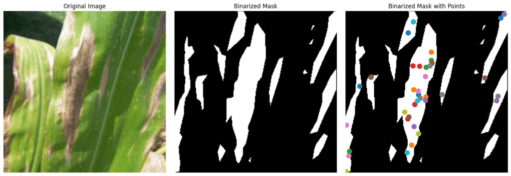
Finally, we rearrange the mask into the shape (1, H, W) and the points into the shape (num_points, 1, 2), preparing them for input into the SAM2 model. This will be our structure of the training batch [input image, mask, the points, and the number of seg masks] for finetuning SAM2, and this is the finest approach to train SAM2 very quickly, with less computational expenses.
Finetuning SAM2 – Building the SAM2 Model
sam2_checkpoint = "../sam2_hiera_tiny.pt"
model_cfg = "sam2_hiera_t.yaml"

sam2_model = build_sam2(model_cfg, sam2_checkpoint, device="cuda")
predictor = SAM2ImagePredictor(sam2_model)

predictor.model.sam_mask_decoder.train(True)
predictor.model.sam_prompt_encoder.train(True)
Here, we specify the paths to the pre-trained checkpoint (sam2_hiera_tiny.pt) and the matching model configuration (sam2_hiera_t.yaml). By initializing build_sam2 with these paths, we instantiate the core SAM2 model on the GPU. The SAM2ImagePredictor class is then created to manage prompts and predictions conveniently. Setting sam_mask_decoder and sam_prompt_encoder to training mode ensures that the relevant layers can be fine-tuned when we start our optimization routine.
P.S. We freeze the image encoder layers to preserve the general visual features learned from massive pre-training and reduce GPU memory usage.
Training Configuration for Finetuning SAM2
scaler = torch.amp.GradScaler()
NO_OF_STEPS = 6000
FINE_TUNED_MODEL_NAME = "fine_tuned_sam2"

optimizer = torch.optim.AdamW(params=predictor.model.parameters(),
                              lr=0.00005,
                              weight_decay=1e-4)

scheduler = torch.optim.lr_scheduler.StepLR(optimizer, step_size=2000, gamma=0.6)
accumulation_steps = 8
To speed up training and potentially reduce memory consumption, we use mixed precision through PyTorch’s GradScaler. We define the total number of training steps and a model name for saving our checkpoints. We have chose AdamW as optimizer, combined with a step learning rate scheduler that reduces the learning rate by a factor (gamma=0.6) every certain number of steps (step_size=2000).
When setting up the training loop, we have to know about a few essential parameters that control how the model learns from the data. These parameters influence how quickly or slowly the model converges, how stable the optimization process is, and ultimately how well the model performs on unseen data. Let’s take a closer look at these tunable parameters and what they do:
Weight Decay (weight_decay = 1e-4) – This parameter adds a penalty to large weights, helping prevent overfitting (type of regularization). It’s particularly useful when the model is prone to memorize the training data rather than generalizing to new inputs.
Gamma (gamma = 0.6) – The gamma value determines the scale of each learning rate reduction. A lower gamma results in a more significant drop in the learning rate, helping fine-tune the model’s parameters more precisely during later stages of training.
Gradient Accumulation Steps (accumulation_steps = 8) – Instead of updating the model’s weights after every mini-batch, this setting allows the optimizer to wait until gradients from multiple mini-batches are accumulated before performing an update. This effectively simulates a larger batch size, which can be beneficial when memory is limited.
Together, these parameters provide a fine level of control over the training process, making it possible to achieve better performance by carefully adjusting each one. Our primary goal is to achieve the best accuracy by tuning these hyperparameters for finetuning SAM2.
Finetuning SAM2 – Training and Validation Loops
Training Function
def train(predictor, train_data, step, mean_iou):
    with torch.amp.autocast(device_type='cuda'):
        image, mask, input_point, num_masks = read_batch(train_data, visualize_data=False)

        if image is None or mask is None or num_masks == 0:
            return

        input_label = np.ones((num_masks, 1))

        if not isinstance(input_point, np.ndarray) or not isinstance(input_label, np.ndarray):
            return

        if input_point.size == 0 or input_label.size == 0:
            return

        predictor.set_image(image)
        mask_input, unnorm_coords, labels, unnorm_box = predictor._prep_prompts(
            input_point, input_label, box=None, mask_logits=None, normalize_coords=True
        )

        if unnorm_coords is None or labels is None or unnorm_coords.shape[0] == 0 or labels.shape[0] == 0:
            return

        sparse_embeddings, dense_embeddings = predictor.model.sam_prompt_encoder(
            points=(unnorm_coords, labels), boxes=None, masks=None
        )

        batched_mode = unnorm_coords.shape[0] > 1
        high_res_features = [feat_level[-1].unsqueeze(0) for feat_level in predictor._features["high_res_feats"]]

        low_res_masks, prd_scores, _, _ = predictor.model.sam_mask_decoder(
            image_embeddings=predictor._features["image_embed"][-1].unsqueeze(0),
            image_pe=predictor.model.sam_prompt_encoder.get_dense_pe(),
            sparse_prompt_embeddings=sparse_embeddings,
            dense_prompt_embeddings=dense_embeddings,
            multimask_output=True,
            repeat_image=batched_mode,
            high_res_features=high_res_features,
        )

        prd_masks = predictor._transforms.postprocess_masks(low_res_masks, predictor._orig_hw[-1])

        gt_mask = torch.tensor(mask.astype(np.float32)).cuda()
        prd_mask = torch.sigmoid(prd_masks[:, 0])

        seg_loss = (-gt_mask * torch.log(prd_mask + 1e-6) - (1 - gt_mask) * torch.log((1 - prd_mask) + 1e-6)).mean()

        inter = (gt_mask * (prd_mask > 0.5)).sum(1).sum(1)
        iou = inter / (gt_mask.sum(1).sum(1) + (prd_mask > 0.5).sum(1).sum(1) - inter)

        score_loss = torch.abs(prd_scores[:, 0] - iou).mean()
        loss = seg_loss + score_loss * 0.05

        loss = loss / accumulation_steps
        scaler.scale(loss).backward()

        torch.nn.utils.clip_grad_norm_(predictor.model.parameters(), max_norm=1.0)

        if step % accumulation_steps == 0:
            scaler.step(optimizer)
            scaler.update()
            predictor.model.zero_grad()

        scheduler.step()

        mean_iou = mean_iou * 0.99 + 0.01 * np.mean(iou.cpu().detach().numpy())

        if step % 100 == 0:
            current_lr = optimizer.param_groups[0]["lr"]
            print(f"Step {step}: Current LR = {current_lr:.6f}, IoU = {mean_iou:.6f}, Seg Loss = {seg_loss:.6f}")
    return mean_iou
In the training function, we start by reading a single random batch (which, in our example, is essentially one image-mask pair at a time). We create a foreground label (input_label = 1) for each set of prompt points. The predictor first encodes the image, then encodes the prompts (_prep_prompts), and finally feeds these embeddings into sam_mask_decoder to obtain the predicted masks.
The model processes these inputs in two main stages: prompt encoding and mask decoding.
First, the prompt encoder takes the input prompt points and their labels (which indicate foreground or background) and encodes them into dense and sparse embeddings. Sparse embeddings are derived from the specific locations of the points, capturing spatial information at a fine level. Dense embeddings, on the other hand, provide a broader representation of the image and the prompts by embedding them into a continuous feature space. This twofold approach allows the model to use precise location data from sparse embeddings while also benefiting from the general contextual information in the dense embeddings.
Once the embeddings are prepared, they are passed to the mask decoder, which generates segmentation masks. The decoder uses these embeddings, along with stored image features and positional encodings, to predict a set of low-resolution masks. These masks are then upsampled and compared against the ground-truth mask using a segmentation loss function. The entire process is designed to refine the model’s ability to correctly identify and segment regions of interest based on the provided point prompts.
Then, we compute two main losses: a binary cross-entropy (BCE) based segmentation loss and a score loss that tries to match the model’s predicted score (essentially a confidence measure) to the ground-truth IoU of the predicted mask. We then divide the loss by accumulation_steps to accumulate gradients over multiple forward passes. After scaling the loss using scaler.scale, we backprop through the network, clip gradients if they exceed a certain norm, and then update the optimizer every time we complete accumulation_steps mini-batches. We also update our learning rate scheduler and maintain a running average of IoU to monitor performance over time.
Validate Function
def validate(predictor, test_data, step, mean_iou):
    predictor.model.eval()
    with torch.amp.autocast(device_type='cuda'):
        with torch.no_grad():
            image, mask, input_point, num_masks = read_batch(test_data, visualize_data=False)

            if image is None or mask is None or num_masks == 0:
                return

            input_label = np.ones((num_masks, 1))

            if not isinstance(input_point, np.ndarray) or not isinstance(input_label, np.ndarray):
                return

            if input_point.size == 0 or input_label.size == 0:
                return

            predictor.set_image(image)
            mask_input, unnorm_coords, labels, unnorm_box = predictor._prep_prompts(
                input_point, input_label, box=None, mask_logits=None, normalize_coords=True
            )

            if unnorm_coords is None or labels is None or unnorm_coords.shape[0] == 0 or labels.shape[0] == 0:
                return

            sparse_embeddings, dense_embeddings = predictor.model.sam_prompt_encoder(
                points=(unnorm_coords, labels), boxes=None, masks=None
            )

            batched_mode = unnorm_coords.shape[0] > 1
            high_res_features = [feat_level[-1].unsqueeze(0) for feat_level in predictor._features["high_res_feats"]]
            low_res_masks, prd_scores, _, _ = predictor.model.sam_mask_decoder(
                image_embeddings=predictor._features["image_embed"][-1].unsqueeze(0),
                image_pe=predictor.model.sam_prompt_encoder.get_dense_pe(),
                sparse_prompt_embeddings=sparse_embeddings,
                dense_prompt_embeddings=dense_embeddings,
                multimask_output=True,
                repeat_image=batched_mode,
                high_res_features=high_res_features,
            )

            prd_masks = predictor._transforms.postprocess_masks(low_res_masks, predictor._orig_hw[-1])

            gt_mask = torch.tensor(mask.astype(np.float32)).cuda()
            prd_mask = torch.sigmoid(prd_masks[:, 0])

            seg_loss = (-gt_mask * torch.log(prd_mask + 1e-6)
                        - (1 - gt_mask) * torch.log((1 - prd_mask) + 1e-6)).mean()

            inter = (gt_mask * (prd_mask > 0.5)).sum(1).sum(1)
            iou = inter / (gt_mask.sum(1).sum(1) + (prd_mask > 0.5).sum(1).sum(1) - inter)

            score_loss = torch.abs(prd_scores[:, 0] - iou).mean()
            loss = seg_loss + score_loss * 0.05
            loss = loss / accumulation_steps

            if step % 500 == 0:
                FINE_TUNED_MODEL = FINE_TUNED_MODEL_NAME + "_" + str(step) + ".pt"
                torch.save(predictor.model.state_dict(), FINE_TUNED_MODEL)

            mean_iou = mean_iou * 0.99 + 0.01 * np.mean(iou.cpu().detach().numpy())

            if step % 100 == 0:
                current_lr = optimizer.param_groups[0]["lr"]
                print(f"Step {step}: Current LR = {current_lr:.6f}, Valid_IoU = {mean_iou:.6f}, Valid_Seg Loss = {seg_loss:.6f}")
    return mean_iou
The validation function is almost identical to the training function, except that we switch the model to evaluation mode (model.eval()) and wrap our forward pass in torch.no_grad(). This ensures that no gradients are calculated or updated and that certain layers (like batch normalization and dropout) behave consistently during inference. We compute a validation loss and IoU to track how well the model performs over our test data, and we save a model checkpoint every 500 steps so that we can run the inference on the fine-tuned model.
Run the Training
train_mean_iou = 0
valid_mean_iou = 0

for step in range(1, NO_OF_STEPS + 1):
    train_mean_iou = train(predictor, train_data, step, train_mean_iou)
    valid_mean_iou = validate(predictor, test_data, step, valid_mean_iou)
In this loop, we repeatedly call train on train_data and validate on test_data. Each iteration processes exactly one sample, so in effect, each “step” is one mini-batch’s worth of data. The NO_OF_STEPS value of 6000 means you’ll cycle many times through the dataset, which is especially suitable if your dataset is not extremely large. Over time, the network’s learned parameters should steadily improve, guided by the computed losses and updated IoU metrics.
After doing all of this we are able to finetune SAM2 on our leaf disease dataset in an 8 GB local GPU. And the training log looks like this:
Step 100: Current LR = 0.000050, IoU = 0.442199, Seg Loss = 0.226500
Step 100: Current LR = 0.000050, Valid_IoU = 0.418000, Valid_Seg Loss = 0.074199
Step 200: Current LR = 0.000050, IoU = 0.615555, Seg Loss = 0.214060
Step 200: Current LR = 0.000050, Valid_IoU = 0.590300, Valid_Seg Loss = 0.050629
.
.
.
Step 1000: Current LR = 0.000050, IoU = 0.732116, Seg Loss = 0.280963
Step 1000: Current LR = 0.000050, Valid_IoU = 0.705820, Valid_Seg Loss = 0.239118
Step 1100: Current LR = 0.000050, IoU = 0.727678, Seg Loss = 0.199423
Step 1100: Current LR = 0.000050, Valid_IoU = 0.700250, Valid_Seg Loss = 0.037643
Step 1200: Current LR = 0.000050, IoU = 0.718707, Seg Loss = 0.189278
Step 1200: Current LR = 0.000050, Valid_IoU = 0.692800, Valid_Seg Loss = 0.126587
.
.
.
Step 2000: Current LR = 0.000030, IoU = 0.707341, Seg Loss = 0.139096
Step 2000: Current LR = 0.000030, Valid_IoU = 0.675010, Valid_Seg Loss = 0.065017
.
.
Step 3000: Current LR = 0.000030, IoU = 0.705332, Seg Loss = 0.712275
Step 3000: Current LR = 0.000030, Valid_IoU = 0.671869, Valid_Seg Loss = 0.006976
.
.
.
Step 6000: Current LR = 0.000005, IoU = 0.747317, Seg Loss = 0.100163
Step 6000: Current LR = 0.000005, Valid_IoU = 0.680088, Valid_Seg Loss = 0.073439
.
.
.
The best IoU we achieved is 68% val IoU. Now, a small task for you: download the code, run the training, apply more strategies, tune the parameters, and achieve a higher accuracy. Let us know in the comments as well.
We use IoU as our primary metric. For a more comprehensive evaluation, you can also track Dice coefficient or pixel accuracy. Additionally, rather than logging IoU after every single iteration (which might be noisy), you can evaluate on the entire validation set at intervals (e.g., every 500 steps or each epoch) to get a more stable measure of generalization.
Inference on Finetuned SAM2
After finetuning SAM2, we do the inference with our fine-tuned model. Let’s see how well our model learned!
def read_image(image_path, mask_path):  # read and resize image and mask
   img = cv2.imread(image_path)[..., ::-1]  # Convert BGR to RGB
   mask = cv2.imread(mask_path, 0)
   r = np.min([1024 / img.shape[1], 1024 / img.shape[0]])
   img = cv2.resize(img, (int(img.shape[1] * r), int(img.shape[0] * r)))
   mask = cv2.resize(mask, (int(mask.shape[1] * r), int(mask.shape[0] * r)), interpolation=cv2.INTER_NEAREST)
   return img, mask

def get_points(mask, num_points):  # Sample points inside the input mask
   points = []
   coords = np.argwhere(mask > 0)
   for i in range(num_points):
       yx = np.array(coords[np.random.randint(len(coords))])
       points.append([[yx[1], yx[0]]])
   return np.array(points)
First, we write two helper functions to process the inputs for inference. The read_image function reads a given image and mask from file paths, then resizes them to a manageable resolution while preserving their aspect ratio. The get_points function, on the other hand, takes a segmentation mask and randomly samples prompt points from within the regions of interest. These points guide the model during inference, helping it understand which parts of the image to focus on.
# Randomly select a test image from the test_data
selected_entry = random.choice(test_data)
.print(selected_entry)
image_path = selected_entry['image']
mask_path = selected_entry['annotation']
print(mask_path,'mask path')

# Load the selected image and mask
image, target_mask = read_image(image_path, mask_path)

# Generate random points for the input
num_samples = 30  # Number of points per segment to sample
input_points = get_points(target_mask, num_samples)

# Load the fine-tuned model
FINE_TUNED_MODEL_WEIGHTS = "../fine_tuned_sam2.pt"
sam2_model = build_sam2(model_cfg, sam2_checkpoint, device="cuda")

# Build net and load weights
predictor = SAM2ImagePredictor(sam2_model)
predictor.model.load_state_dict(torch.load(FINE_TUNED_MODEL_WEIGHTS))


# Perform inference and predict masks
with torch.no_grad():
   predictor.set_image(image)
   masks, scores, logits = predictor.predict(
       point_coords=input_points,
       point_labels=np.ones([input_points.shape[0], 1])
   )

# Process the predicted masks and sort by scores
np_masks = np.array(masks[:, 0])
np_scores = scores[:, 0]
sorted_masks = np_masks[np.argsort(np_scores)][::-1]

# Initialize segmentation map and occupancy mask
seg_map = np.zeros_like(sorted_masks[0], dtype=np.uint8)
occupancy_mask = np.zeros_like(sorted_masks[0], dtype=bool)

# Combine masks to create the final segmentation map
for i in range(sorted_masks.shape[0]):
   mask = sorted_masks[i]
   if (mask * occupancy_mask).sum() / mask.sum() > 0.15:
       continue

   mask_bool = mask.astype(bool)
   mask_bool[occupancy_mask] = False  # Set overlapping areas to False in the mask
   seg_map[mask_bool] = i + 1  # Use boolean mask to index seg_map
   occupancy_mask[mask_bool] = True  # Update occupancy_mask

# Visualization: Show the original image, mask, and final segmentation side by side
plt.figure(figsize=(18, 6))

plt.subplot(1, 3, 1)
plt.title('Test Image')
plt.imshow(image)
plt.axis('off')

plt.subplot(1, 3, 2)
plt.title('Original Mask')
plt.imshow(target_mask, cmap='gray')
plt.axis('off')

plt.subplot(1, 3, 3)
plt.title('Final Segmentation')
plt.imshow(seg_map, cmap='jet')
plt.axis('off')

plt.tight_layout()
plt.show()
When running inference, we start by selecting a random test sample, load its image and mask, and using get_points utility to extract prompt points. The saved weights of the fine-tuned SAM2 model are then loaded into the predictor, which is initialized with the corresponding configuration. Once the model is prepared, we pass the image and prompt points into the predictor’s predict method. SAM2 is prompt-driven, so at inference time we must provide at least one prompt (in this case, a point). This returns the predicted masks, scores, and logits, all of which can be used to build the final segmentation output.
The visualization step takes the outputs and compares them to the ground truth. First, the predicted masks are sorted by their confidence scores, and we merge them into a final segmentation map. We ensure that the resulting segmentation is clean and non-redundant by skipping overlapping regions that less a certain threshold. Finally, we plot the original image, the ground-truth mask, and the generated segmentation map side by side, providing a clear visual comparison of the model’s performance.
Now let’s see some of the inference results:
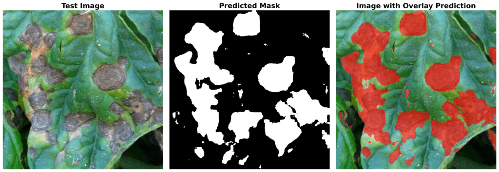
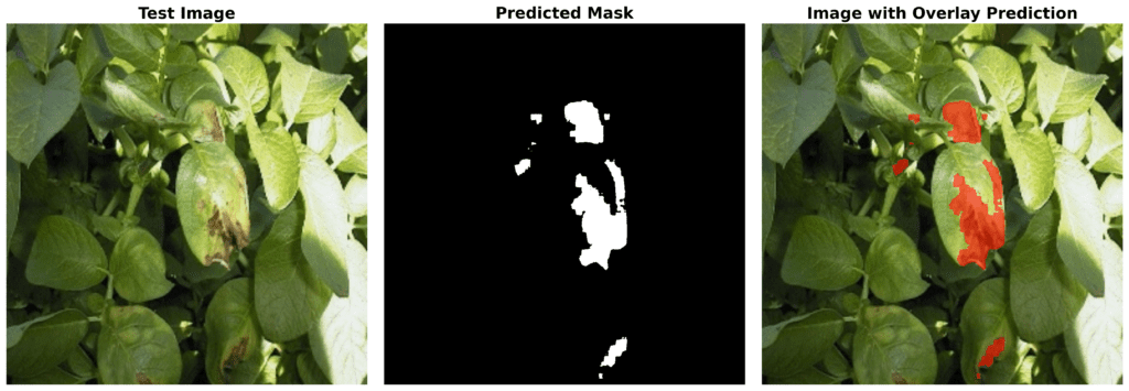
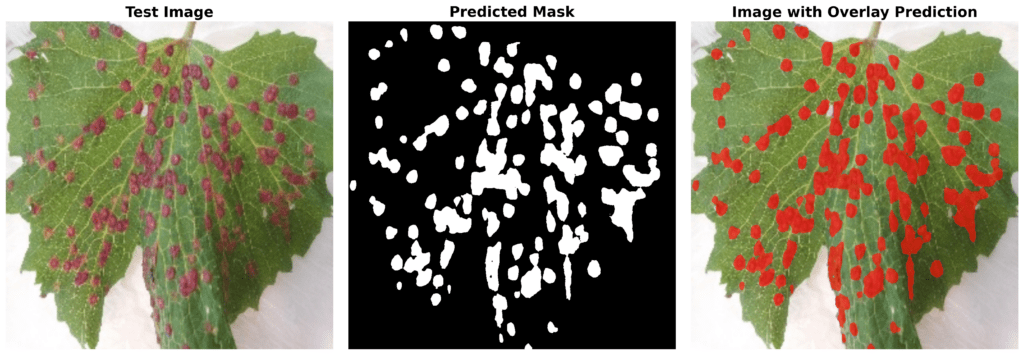
But there is a question: Why do we need to pass the mask with points during inference if we have already finetuned the model?
During training, the model learns to interpret prompts (such as points) and generate segmentation masks. The main purpose of training with points and their corresponding labels is to teach the model how to respond to prompts effectively. However, during inference, even though the model is already trained, it still needs input prompts to guide its predictions. The prompts help the model identify the specific region of interest in the image, especially when the image might contain multiple objects or areas.
By providing the mask with points, you’re essentially specifying “look here” so that the model knows where to focus. Without these prompts, the model wouldn’t have any explicit instruction on what part of the image to segment. In essence, the prompts are not there because the model still needs to learn—they are there because they are an inherent part of how the model makes decisions after being trained. This approach allows for flexible, targeted segmentation in varying scenarios.
Now let’s compare the results with pre-trained the SAM2 predictions:
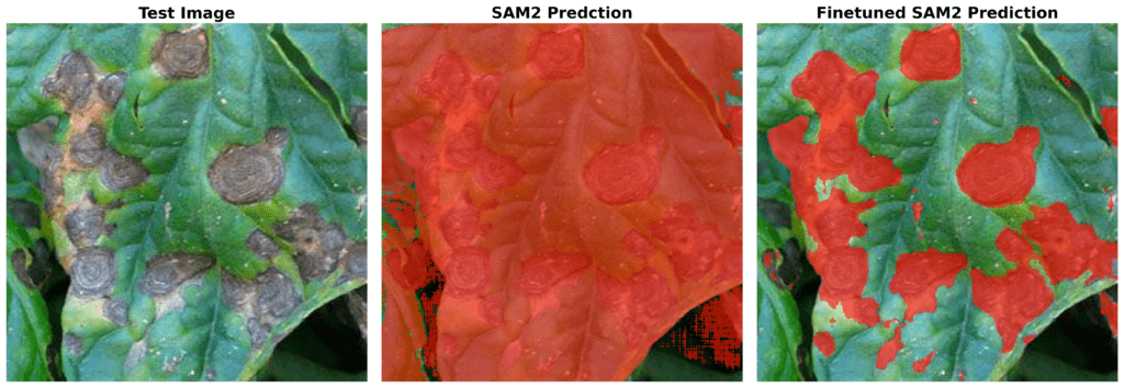
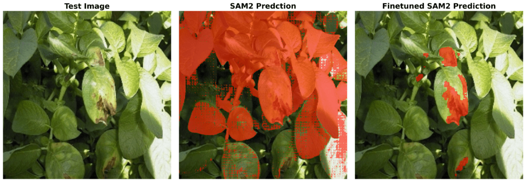
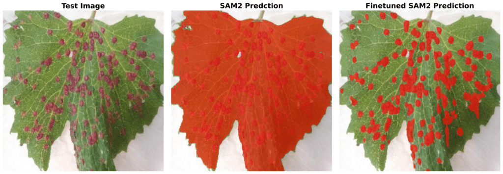
Now, you can understand how important it is to train SAM2 for this specific task. Although SAM2 is trained on billion images, it’s not able to detect the diseased parts without finetuning. But, after fine-tuning SAM2 with this small data and just for 6000 steps, meaningful results.
As we are almost at the end of our article, let’s quickly look at what we have covered.
Quick Recap – Finetuing SAM2
1. Understanding Leaf Disease Segmentation and Its Challenges
Leaf disease segmentation helps detect and isolate diseased crop areas, reducing economic losses and improving food security. Challenges include limited publicly available segmentation datasets, the need for early detection, and ensuring models generalize well across different plant species.
2. Why SAM2 for This Task?
SAM2 is built for promptable segmentation, allowing flexible object detection using points, bounding boxes, or masks. It is pre-trained on a large-scale dataset (SA-V) and can perform zero-shot segmentation, making it effective even with limited labeled data.
3. Training Strategy for SAM2
The fine-tuning approach involves using points as prompts along with binary masks. The dataset is preprocessed into an optimal structure, and a carefully designed training loop incorporates gradient accumulation, loss balancing, and adaptive learning rate adjustments to optimize performance while maintaining computational efficiency.
4. Results and Performance Evaluation
The fine-tuned SAM2 model achieved a 74% train IoU on the leaf disease segmentation dataset. The inference shows satisfactory results, showing the model’s ability to generalize with minimal fine-tuning using a standard 8GB Nvidia Geforce RTX 3070 Ti GPU.
Conclusion
Finetuning SAM2 for Leaf Disease Segmentation provides an efficient approach to identifying and segmenting diseased areas in crops. With limited segmentation datasets available, SAM2’s prompt-based approach enables effective adaptation to this domain. The fine-tuned model delivers reliable performance on a small dataset, achieving an IoU of 74%. Future improvements can focus on optimizing prompt strategies, experimenting with larger datasets, and exploring real-time deployment in agricultural monitoring systems.
If you achieve better accuracy by experimenting with the code, let us know in the comments. See you in the next blog!
References
Meta Segment Anything Model 2 (SAM 2)
Fine-Tuning SAM 2 on a Custom Dataset: Tutorial






100K+ Learners
Join Free OpenCV Bootcamp3 Hours of Learning