Since its inception, the YOLO family of object detection models has come a long way. YOLOv7 is the most recent addition to this famous anchor-based single-shot family of object detectors. It comes with a bunch of improvements which include state-of-the-art accuracy and speed. In this article, we will be fine tuning the YOLOv7 object detection model on a real-world pothole detection dataset.
Benchmarked on the COCO dataset, the YOLOv7 tiny model achieves more than 35% mAP and the YOLOv7 (normal) model achieves more than 51% mAP. It is also equally important that we get good results when fine tuning such a state-of-the-art model. For that reason, we will be fine tuning YOLOv7 on a real-world pothole detection dataset in this blog post.

| If you are completely new to YOLOv7, it is highly recommended that you go through the article YOLOv7 Object Detection Paper Explanation and Inference. This introductory article covers the following. 1. The details about the YOLOv7 architecture 2. The training experiments and results from the YOLOv7 paper 3. Running inference using YOLOv7 for object detection 4. Running inference using YOLOv7 for human pose estimation |
- Brief About the Pothole Detection Dataset
- The Training Experiments that We Will Carry Out
- Fine Tuning YOLOv7 on the Pothole Detection Dataset
- Running Inference using the Trained Models
- Conclusion
YOLO Master Post – Every Model Explained
Don’t miss out on this comprehensive resource, Mastering All Yolo Models for a richer, more informed perspective on the YOLO series.
1. Brief About the Pothole Detection Dataset
In this blog post, we will use a pothole detection dataset which is a combination of two datasets. We have already discussed the details of the dataset in one of the previous posts. Here, we will go over some of the important points and the changes that we have made.
The dataset consists of images from two different sources. They are
- The Roboflow pothole detection dataset.
- Pothole dataset that is mentioned in this ResearchGate article – Dataset of images used for pothole detection.
After combining, the dataset now contains:
- 1265 training images
- 401 validation images
- 118 test images
Compared to the previous YOLOv4 pothole training post, the dataset in this post has a slight variation in images. All the images which were greater than 1500 pixels in height have been downsampled by a factor of 0.3. This brings all the images to a normalized resolution of almost the same factor.
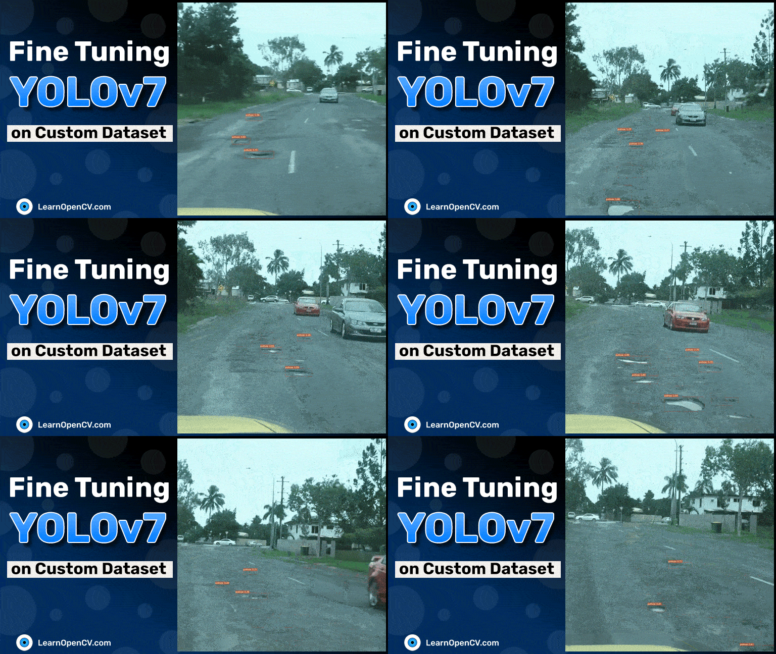
The following are a few of the annotated images from the dataset.
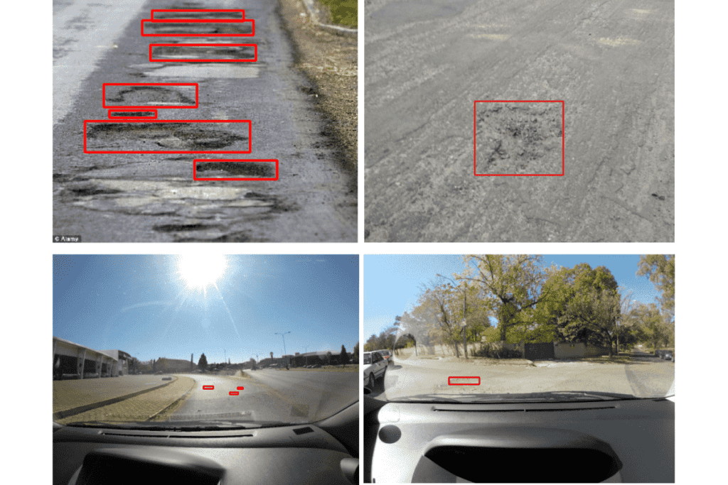
Images from the pothole detection dataset that we will use for fine tuning YOLOv7.
The dataset contains images from car dashboard cameras and also photos taken from handheld cameras on roads.
2. The Training Experiments that We Will Carry Out
We will carry out four training experiments using the YOLOv7 models in this blog post.
- We will start with fine tuning the YOLOv7 tiny model with fixed resolution.
- Then we will move on to training the YOLOv7 tiny model using multi-resolution images.
- Next, we will train the YOLOv7 model with fixed-resolution images.
- Finally, we will train the YOLOv7 model on multi-resolution images.
We will get into the details of all the training settings, parameters, and models in their respective training sections. Fine tuning a YOLOv7 model has its own intricacies that require some attention. But we will cover all the points in detail as we move through the model training sections.
Don’t miss out on the new YOLOv6 paper explanation and inference post. You will learn about the model architecture, how it is industrial application ready, and how it performs during inference.
3. Fine Tuning YOLOv7 on the Pothole Detection Dataset
The training steps that we will follow are meant to be executed in a Jupyter notebook. A one-click runnable Jupyter notebook is provided in the download section of this post. Although we will cover only the dataset preparation and training parts of the code here, the Jupyter notebook also contains code for data visualization which you can use for exploring the dataset in depth.
If you are on Ubuntu OS, you can directly run it locally, although you will need a GPU for training the models. If you are on Windows OS, you can run the notebook on Colab which already provides free GPU.
Note: If you run the training experiments, it is highly recommended to use a GPU. The training experiments for this blog post were run in a Colab environment using 16 GB Tesla P100 GPU. Your training time may vary depending on the GPU that you use.
From the next section onward, we will start with the downloading of the dataset and setting up YOLOv7 for training. Then we will move into each of the training experiments.
Downloading, and Extracting the Dataset
The very first step is to download and prepare the dataset and all the data files that we will need for training.
The following command downloads the dataset
# Download the dataset.
!wget https://learnopencv.s3.us-west-2.amazonaws.com/pothole_dataset.zip
Let’s extract the dataset and take a look at its directory structure.
# Extract the dataset.
!unzip -q pothole_dataset.zip
pothole_dataset/
├── images
│   ├── test [118 entries exceeds filelimit, not opening dir]
│   ├── train [1265 entries exceeds filelimit, not opening dir]
│   └── valid [401 entries exceeds filelimit, not opening dir]
└── labels
    ├── test [118 entries exceeds filelimit, not opening dir]
    ├── train [1265 entries exceeds filelimit, not opening dir]
    ├── valid [401 entries exceeds filelimit, not opening dir]
We need the images and labels to be in the above directory structure for training YOLOv7. All the images are in their respective directories and all the labels are in their respective labels directories. Every image has a separate text file containing the class label and annotations for each object in a new line. The following is an example.
0 0.5497282608695652 0.5119565217391304 0.017934782608695653 0.005072463768115942
0 0.41032608695652173 0.5253623188405797 0.025 0.005797101449275362
0 0.30842391304347827 0.5282608695652173 0.014673913043478261 0.005797101449275362
0 0.1654891304347826 0.5224637681159421 0.027717391304347826 0.005797101449275362
0 0.10163043478260869 0.5286231884057971 0.01956521739130435 0.006521739130434782
0 0.07907608695652174 0.5293478260869565 0.01576086956521739 0.007971014492753623
The first number is the class label. As we have only one class here, the number is 0. The rest are the bounding box coordinates in <x_center, y_center, width, height> format. All the bounding box coordinates are normalized according to the image size.
Clone the YOLOv7 Repository
The next step is to clone the YOLOv7 repository so that we can access the codebase for training the models.
if not os.path.exists('yolov7'):
    !git clone https://github.com/WongKinYiu/yolov7.git

%cd yolov7

!pip install -r requirements.txt
In the above code block, we clone the YOLOv7 repository if not already present in the current directory. Then we enter the directory and install the requirements.
Creating the Dataset YAML File
Like many of the recent YOLO versions, we will need a dataset YAML file to train any of the YOLOv7 models. This .yaml file contains the paths to the image sets, the number of classes, and the name of the classes.
This file will go into the yolov7/data directory.
%%writefile data/pothole.yaml
train: ../pothole_dataset/images/train
val: ../pothole_dataset/images/valid
test: ../pothole_dataset/images/test

# Classes
nc: 1  # number of classes
names: ['pothole']  # class names
The above code block creates a pothole.yaml file. This contains the paths to the training, validation, and test image. As we are executing the code within the yolov7 directory, the paths are relative to that directory.
If you have worked with YOLOv5, you may observe that the YAML file structure for YOLOv7 is very similar to that of the YOLOv5 dataset YAML file.
3.1 Tiny YOLOv7 Model Fixed Resolution Training
In this section, we will train the YOLOv7-Tiny model. The tiny model contains just over 6 million parameters. We will use the native base resolution images for training the model, which is 640×640. But before we can start the training, there are a few other details that we need to take care of.
First, we need to download the YOLOv7-tiny model.
# Download the Tiny model weights.
!wget https://github.com/WongKinYiu/yolov7/releases/download/v0.1/yolov7-tiny.pt
This will download the latest version of the YOLOv7-tiny model which has been pre-trained on the COCO dataset.
Next, we need to configure the YOLOv7-tiny model for pothole detection training. There are several default configuration files inside yolov7/cfg/training/ directory. All these contain the model configuration. We need to configure the yolov7-tiny.yaml file. For that, we will create a copy of that file, rename it, and configure it accordingly.
The following code block creates a yolov7_pothole-tiny.yaml file.
%%writefile cfg/training/yolov7_pothole-tiny.yaml
# parameters
nc: 1  # number of classes
depth_multiple: 1.0  # model depth multiple
width_multiple: 1.0  # layer channel multiple

# anchors
anchors:
  - [10,13, 16,30, 33,23]  # P3/8
  - [30,61, 62,45, 59,119]  # P4/16
  - [116,90, 156,198, 373,326]  # P5/32

# yolov7-tiny backbone
backbone:
  # [from, number, module, args] c2, k=1, s=1, p=None, g=1, act=True
  [[-1, 1, Conv, [32, 3, 2, None, 1, nn.LeakyReLU(0.1)]],  # 0-P1/2

  [-1, 1, Conv, [64, 3, 2, None, 1, nn.LeakyReLU(0.1)]],  # 1-P2/4

  [-1, 1, Conv, [32, 1, 1, None, 1, nn.LeakyReLU(0.1)]],
  [-2, 1, Conv, [32, 1, 1, None, 1, nn.LeakyReLU(0.1)]],
  [-1, 1, Conv, [32, 3, 1, None, 1, nn.LeakyReLU(0.1)]],
  [-1, 1, Conv, [32, 3, 1, None, 1, nn.LeakyReLU(0.1)]],
  [[-1, -2, -3, -4], 1, Concat, [1]],
  [-1, 1, Conv, [64, 1, 1, None, 1, nn.LeakyReLU(0.1)]],  # 7

  [-1, 1, MP, []],  # 8-P3/8
  [-1, 1, Conv, [64, 1, 1, None, 1, nn.LeakyReLU(0.1)]],
  [-2, 1, Conv, [64, 1, 1, None, 1, nn.LeakyReLU(0.1)]],
  [-1, 1, Conv, [64, 3, 1, None, 1, nn.LeakyReLU(0.1)]],
  [-1, 1, Conv, [64, 3, 1, None, 1, nn.LeakyReLU(0.1)]],
  [[-1, -2, -3, -4], 1, Concat, [1]],
  [-1, 1, Conv, [128, 1, 1, None, 1, nn.LeakyReLU(0.1)]],  # 14

  [-1, 1, MP, []],  # 15-P4/16
  [-1, 1, Conv, [128, 1, 1, None, 1, nn.LeakyReLU(0.1)]],
  [-2, 1, Conv, [128, 1, 1, None, 1, nn.LeakyReLU(0.1)]],
  [-1, 1, Conv, [128, 3, 1, None, 1, nn.LeakyReLU(0.1)]],
  [-1, 1, Conv, [128, 3, 1, None, 1, nn.LeakyReLU(0.1)]],
  [[-1, -2, -3, -4], 1, Concat, [1]],
  [-1, 1, Conv, [256, 1, 1, None, 1, nn.LeakyReLU(0.1)]],  # 21

  [-1, 1, MP, []],  # 22-P5/32
  [-1, 1, Conv, [256, 1, 1, None, 1, nn.LeakyReLU(0.1)]],
  [-2, 1, Conv, [256, 1, 1, None, 1, nn.LeakyReLU(0.1)]],
  [-1, 1, Conv, [256, 3, 1, None, 1, nn.LeakyReLU(0.1)]],
  [-1, 1, Conv, [256, 3, 1, None, 1, nn.LeakyReLU(0.1)]],
  [[-1, -2, -3, -4], 1, Concat, [1]],
  [-1, 1, Conv, [512, 1, 1, None, 1, nn.LeakyReLU(0.1)]],  # 28
  ]

# yolov7-tiny head
head:
  [[-1, 1, Conv, [256, 1, 1, None, 1, nn.LeakyReLU(0.1)]],
  [-2, 1, Conv, [256, 1, 1, None, 1, nn.LeakyReLU(0.1)]],
  [-1, 1, SP, [5]],
  [-2, 1, SP, [9]],
  [-3, 1, SP, [13]],
  [[-1, -2, -3, -4], 1, Concat, [1]],
  [-1, 1, Conv, [256, 1, 1, None, 1, nn.LeakyReLU(0.1)]],
  [[-1, -7], 1, Concat, [1]],
  [-1, 1, Conv, [256, 1, 1, None, 1, nn.LeakyReLU(0.1)]],  # 37

  [-1, 1, Conv, [128, 1, 1, None, 1, nn.LeakyReLU(0.1)]],
  [-1, 1, nn.Upsample, [None, 2, 'nearest']],
  [21, 1, Conv, [128, 1, 1, None, 1, nn.LeakyReLU(0.1)]], # route backbone P4
  [[-1, -2], 1, Concat, [1]],

  [-1, 1, Conv, [64, 1, 1, None, 1, nn.LeakyReLU(0.1)]],
  [-2, 1, Conv, [64, 1, 1, None, 1, nn.LeakyReLU(0.1)]],
  [-1, 1, Conv, [64, 3, 1, None, 1, nn.LeakyReLU(0.1)]],
  [-1, 1, Conv, [64, 3, 1, None, 1, nn.LeakyReLU(0.1)]],
  [[-1, -2, -3, -4], 1, Concat, [1]],
  [-1, 1, Conv, [128, 1, 1, None, 1, nn.LeakyReLU(0.1)]],  # 47

  [-1, 1, Conv, [64, 1, 1, None, 1, nn.LeakyReLU(0.1)]],
  [-1, 1, nn.Upsample, [None, 2, 'nearest']],
  [14, 1, Conv, [64, 1, 1, None, 1, nn.LeakyReLU(0.1)]], # route backbone P3
  [[-1, -2], 1, Concat, [1]],

  [-1, 1, Conv, [32, 1, 1, None, 1, nn.LeakyReLU(0.1)]],
  [-2, 1, Conv, [32, 1, 1, None, 1, nn.LeakyReLU(0.1)]],
  [-1, 1, Conv, [32, 3, 1, None, 1, nn.LeakyReLU(0.1)]],
  [-1, 1, Conv, [32, 3, 1, None, 1, nn.LeakyReLU(0.1)]],
  [[-1, -2, -3, -4], 1, Concat, [1]],
  [-1, 1, Conv, [64, 1, 1, None, 1, nn.LeakyReLU(0.1)]],  # 57

  [-1, 1, Conv, [128, 3, 2, None, 1, nn.LeakyReLU(0.1)]],
  [[-1, 47], 1, Concat, [1]],

  [-1, 1, Conv, [64, 1, 1, None, 1, nn.LeakyReLU(0.1)]],
  [-2, 1, Conv, [64, 1, 1, None, 1, nn.LeakyReLU(0.1)]],
  [-1, 1, Conv, [64, 3, 1, None, 1, nn.LeakyReLU(0.1)]],
  [-1, 1, Conv, [64, 3, 1, None, 1, nn.LeakyReLU(0.1)]],
  [[-1, -2, -3, -4], 1, Concat, [1]],
  [-1, 1, Conv, [128, 1, 1, None, 1, nn.LeakyReLU(0.1)]],  # 65

  [-1, 1, Conv, [256, 3, 2, None, 1, nn.LeakyReLU(0.1)]],
  [[-1, 37], 1, Concat, [1]],

  [-1, 1, Conv, [128, 1, 1, None, 1, nn.LeakyReLU(0.1)]],
  [-2, 1, Conv, [128, 1, 1, None, 1, nn.LeakyReLU(0.1)]],
  [-1, 1, Conv, [128, 3, 1, None, 1, nn.LeakyReLU(0.1)]],
  [-1, 1, Conv, [128, 3, 1, None, 1, nn.LeakyReLU(0.1)]],
  [[-1, -2, -3, -4], 1, Concat, [1]],
  [-1, 1, Conv, [256, 1, 1, None, 1, nn.LeakyReLU(0.1)]],  # 73

  [57, 1, Conv, [128, 3, 1, None, 1, nn.LeakyReLU(0.1)]],
  [65, 1, Conv, [256, 3, 1, None, 1, nn.LeakyReLU(0.1)]],
  [73, 1, Conv, [512, 3, 1, None, 1, nn.LeakyReLU(0.1)]],

  [[74,75,76], 1, IDetect, [nc, anchors]],   # Detect(P3, P4, P5)
  ]
For our purpose, we only need to change the number of classes (nc) to 1. All other configurations remain the same. We can also see the model architecture for the YOLOv7-tiny model. We will need this file while training to load the proper model architecture.
Executing the Training Command
Next, we will execute the command to train the model.
!python train.py --epochs 100 --workers 4 --device 0 --batch-size 32 \
--data data/pothole.yaml --img 640 640 --cfg cfg/training/yolov7_pothole-tiny.yaml \
--weights 'yolov7-tiny.pt' --name yolov7_tiny_pothole_fixed_res --hyp data/hyp.scratch.tiny.yaml
Let’s go over the important flags in the above command:
--device: The GPU number (ID) to use for training. As we have only one GPU, so, it is 0.
--data: This accepts the path to the dataset YAML file.--img: By default, the images will be resized to 640×640 resolution before being fed to the network. Still, we are providing the image size here.--cfg: This is the path to the model configuration file which is needed for loading the model architecture which we created just before.--weights: This flag accepts the path to the pretrained model.--name: All the training, validation, and test results are saved in subdirectories inside the runs directory by default. We can provide the name of these subdirectories by specifying a string name from this flag.--hyp: All the models in the YOLOv7 family have a different set of parameters and hyperparameters. These include the learning rate, the augmentation techniques, and also the intensity of the augmentations among many other hyperparameters. All these are defined in their hyperparameter files (YAML files) in the yolov7/data directory. Here, we specify the path to the appropriate YOLOv7-tiny model hyperparameter file.
The other flags define the number of epochs to train for, the batch size, and the number of workers. You can set these according to the hardware that you are using. Here, we are training the model for 100 epochs.
The following are the results after 100 epochs.
Epoch   gpu_mem       box       obj       cls     total    labels  img_size
    99/99     4.66G   0.02915   0.00714         0   0.03629        50       640: 100% 40/40 [01:38<00:00,  2.45s/it]
              Class      Images      Labels           P           R      mAP@.5  mAP@.5:.95: 100% 7/7 [00:12<00:00,  1.77s/it]
                all         401        1034       0.689       0.624        0.65       0.322
On the validation set, we have a mAP of 0.65 at 0.5 IoU and 0.322 at 0.5:0.95 IoU. We can also check the precision on the test set using the trained model using the following command.

Results after fine tuning YOLOv7-tiny model on the pothole detection dataset.
Considering that we trained a small model, this looks good. Let’s take a
!python test.py --weights runs/train/yolov7_tiny_pothole_fixed_res/weights/best.pt --task test --data data/pothole.yaml
Class      Images      Labels           P           R      mAP@.5  mAP@.5:.95: 100% 4/4 [00:04<00:00,  1.09s/it]
                all         118         304        0.82       0.556        0.64       0.348
We are getting mAP of 0.64 and 0.348 respectively on the test dataset.
3.2 Tiny YOLOv7 Model Multi-Resolution Training
YOLOv7 also provides the option to train using multi-resolution images. Unlike the previous training experiment, where we used a fixed resolution of 640×640, the size of the images will be varied every few batches.
In multi-resolution training, we need to provide the base resolution (say, 640×640). During training, the images will be resized to +-50% if this base resolution. So, for 640×640 images, the minimum resolution will be 320×320 and the maximum resolution will be 1280×1280. Generally, this helps to train a more robust model especially for cases when we have smaller objects, like this dataset. But we also need to train for longer as the dataset becomes much more difficult because of the varied sizes.
Executing the Training Command
We just have to add one extra flag to the training command to train a multi-scale model.
!python train.py --epochs 100 --workers 4 --device 0 --batch-size 32 \
--data data/pothole.yaml --img 640 640 --cfg cfg/training/yolov7_pothole-tiny.yaml \
--weights 'yolov7-tiny.pt' --name yolov7_tiny_pothole_multi_res --hyp data/hyp.scratch.tiny.yaml \
--multi-scale
As you can see, everything remains the same, except that we add one –multi-scale flag to carry out the multi-resolution training.
The following are the final epoch’s results.
Epoch   gpu_mem       box       obj       cls     total    labels  img_size
99/99     12.6G   0.03214   0.01051         0   0.04265        50       896
Class      Images      Labels           P           R      mAP@.5  mAP@.5:.95: 100% 7/7 [00:12<00:00,  1.77s/it]
all         401     0.757    0.5725    0.6255      0.31
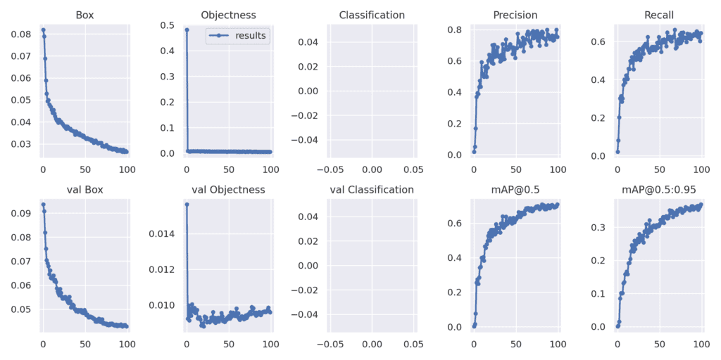
Fine tuning results for YOLOv7-tiny multi-resolution training.
As you may observe, there are a few more dips compared to the fixed-resolution training.
Also, let’s check the test results.
!python test.py --weights runs/train/yolov7_tiny_pothole_multi_res/weights/best.pt --task test --data data/pothole.yaml
Class      Images      Labels           P           R      mAP@.5  mAP@.5:.95: 100% 4/4 [00:04<00:00,  1.04s/it]
                all         118         304       0.707       0.605       0.624       0.351
This time, we have a lower mAP at 0.5 IoU. This can be attributed to the varying image sizes during training. If we train for even longer, these results will be even better. We will get more insights when running inference using the trained models.
3.3 YOLOv7 Fixed Resolution Training
Now, we will start the training experiments using the YOLOv7 normal model. The authors call this one just YOLOv7 and we will refer to it using the same name. This model is much larger compared to the tiny model, containing 37 million parameters. We can surely expect it to give better results than the previous training experiments.
We will need to do a few similar setups as we did for the tiny model. The first step is downloading the YOLOv7 pre-trained model.
!wget https://github.com/WongKinYiu/yolov7/releases/download/v0.1/yolov7_training.pt
Then creating the model configuration file for the custom dataset.
%%writefile cfg/training/yolov7_pothole.yaml
# parameters
nc: 1  # number of classes
depth_multiple: 1.0  # model depth multiple
width_multiple: 1.0  # layer channel multiple

# anchors
anchors:
  - [12,16, 19,36, 40,28]  # P3/8
  - [36,75, 76,55, 72,146]  # P4/16
  - [142,110, 192,243, 459,401]  # P5/32

# yolov7 backbone
backbone:
  # [from, number, module, args]
  [[-1, 1, Conv, [32, 3, 1]],  # 0

  [-1, 1, Conv, [64, 3, 2]],  # 1-P1/2
  [-1, 1, Conv, [64, 3, 1]],

  [-1, 1, Conv, [128, 3, 2]],  # 3-P2/4
  [-1, 1, Conv, [64, 1, 1]],
  [-2, 1, Conv, [64, 1, 1]],
  [-1, 1, Conv, [64, 3, 1]],
  [-1, 1, Conv, [64, 3, 1]],
  [-1, 1, Conv, [64, 3, 1]],
  [-1, 1, Conv, [64, 3, 1]],
  [[-1, -3, -5, -6], 1, Concat, [1]],
  [-1, 1, Conv, [256, 1, 1]],  # 11

  [-1, 1, MP, []],
  [-1, 1, Conv, [128, 1, 1]],
  [-3, 1, Conv, [128, 1, 1]],
  [-1, 1, Conv, [128, 3, 2]],
  [[-1, -3], 1, Concat, [1]],  # 16-P3/8
  [-1, 1, Conv, [128, 1, 1]],
  [-2, 1, Conv, [128, 1, 1]],
  [-1, 1, Conv, [128, 3, 1]],
  [-1, 1, Conv, [128, 3, 1]],
  [-1, 1, Conv, [128, 3, 1]],
  [-1, 1, Conv, [128, 3, 1]],
  [[-1, -3, -5, -6], 1, Concat, [1]],
  [-1, 1, Conv, [512, 1, 1]],  # 24

  [-1, 1, MP, []],
  [-1, 1, Conv, [256, 1, 1]],
  [-3, 1, Conv, [256, 1, 1]],
  [-1, 1, Conv, [256, 3, 2]],
  [[-1, -3], 1, Concat, [1]],  # 29-P4/16
  [-1, 1, Conv, [256, 1, 1]],
  [-2, 1, Conv, [256, 1, 1]],
  [-1, 1, Conv, [256, 3, 1]],
  [-1, 1, Conv, [256, 3, 1]],
  [-1, 1, Conv, [256, 3, 1]],
  [-1, 1, Conv, [256, 3, 1]],
  [[-1, -3, -5, -6], 1, Concat, [1]],
  [-1, 1, Conv, [1024, 1, 1]],  # 37

  [-1, 1, MP, []],
  [-1, 1, Conv, [512, 1, 1]],
  [-3, 1, Conv, [512, 1, 1]],
  [-1, 1, Conv, [512, 3, 2]],
  [[-1, -3], 1, Concat, [1]],  # 42-P5/32
  [-1, 1, Conv, [256, 1, 1]],
  [-2, 1, Conv, [256, 1, 1]],
  [-1, 1, Conv, [256, 3, 1]],
  [-1, 1, Conv, [256, 3, 1]],
  [-1, 1, Conv, [256, 3, 1]],
  [-1, 1, Conv, [256, 3, 1]],
  [[-1, -3, -5, -6], 1, Concat, [1]],
  [-1, 1, Conv, [1024, 1, 1]],  # 50
  ]

# yolov7 head
head:
  [[-1, 1, SPPCSPC, [512]], # 51

  [-1, 1, Conv, [256, 1, 1]],
  [-1, 1, nn.Upsample, [None, 2, 'nearest']],
  [37, 1, Conv, [256, 1, 1]], # route backbone P4
  [[-1, -2], 1, Concat, [1]],

  [-1, 1, Conv, [256, 1, 1]],
  [-2, 1, Conv, [256, 1, 1]],
  [-1, 1, Conv, [128, 3, 1]],
  [-1, 1, Conv, [128, 3, 1]],
  [-1, 1, Conv, [128, 3, 1]],
  [-1, 1, Conv, [128, 3, 1]],
  [[-1, -2, -3, -4, -5, -6], 1, Concat, [1]],
  [-1, 1, Conv, [256, 1, 1]], # 63

  [-1, 1, Conv, [128, 1, 1]],
  [-1, 1, nn.Upsample, [None, 2, 'nearest']],
  [24, 1, Conv, [128, 1, 1]], # route backbone P3
  [[-1, -2], 1, Concat, [1]],

  [-1, 1, Conv, [128, 1, 1]],
  [-2, 1, Conv, [128, 1, 1]],
  [-1, 1, Conv, [64, 3, 1]],
  [-1, 1, Conv, [64, 3, 1]],
  [-1, 1, Conv, [64, 3, 1]],
  [-1, 1, Conv, [64, 3, 1]],
  [[-1, -2, -3, -4, -5, -6], 1, Concat, [1]],
  [-1, 1, Conv, [128, 1, 1]], # 75

  [-1, 1, MP, []],
  [-1, 1, Conv, [128, 1, 1]],
  [-3, 1, Conv, [128, 1, 1]],
  [-1, 1, Conv, [128, 3, 2]],
  [[-1, -3, 63], 1, Concat, [1]],

  [-1, 1, Conv, [256, 1, 1]],
  [-2, 1, Conv, [256, 1, 1]],
  [-1, 1, Conv, [128, 3, 1]],
  [-1, 1, Conv, [128, 3, 1]],
  [-1, 1, Conv, [128, 3, 1]],
  [-1, 1, Conv, [128, 3, 1]],
  [[-1, -2, -3, -4, -5, -6], 1, Concat, [1]],
  [-1, 1, Conv, [256, 1, 1]], # 88

  [-1, 1, MP, []],
  [-1, 1, Conv, [256, 1, 1]],
  [-3, 1, Conv, [256, 1, 1]],
  [-1, 1, Conv, [256, 3, 2]],
  [[-1, -3, 51], 1, Concat, [1]],

  [-1, 1, Conv, [512, 1, 1]],
  [-2, 1, Conv, [512, 1, 1]],
  [-1, 1, Conv, [256, 3, 1]],
  [-1, 1, Conv, [256, 3, 1]],
  [-1, 1, Conv, [256, 3, 1]],
  [-1, 1, Conv, [256, 3, 1]],
  [[-1, -2, -3, -4, -5, -6], 1, Concat, [1]],
  [-1, 1, Conv, [512, 1, 1]], # 101

  [75, 1, RepConv, [256, 3, 1]],
  [88, 1, RepConv, [512, 3, 1]],
  [101, 1, RepConv, [1024, 3, 1]],

  [[102,103,104], 1, IDetect, [nc, anchors]],   # Detect(P3, P4, P5)
  ]
It is clear from the above configuration file that the model contains more layers compared to the tiny model.
Executing the Training Command
!python train.py --epochs 100 --workers 4 --device 0 --batch-size 16 --data data/pothole.yaml \
--img 640 640 --cfg cfg/training/yolov7_pothole.yaml --weights 'yolov7_training.pt' \
--name yolov7_pothole_fixed_res --hyp data/hyp.scratch.custom.yaml
As YOLOv7 is a much larger model, we are using a batch size of 16 to accommodate for the GPU memory usage. Other than that we also configure the –weights, –name, and –hyp flags accordingly.
The following shows the results after the last epoch.
Epoch   gpu_mem       box       obj       cls     total    labels  img_size
    99/99     15.5G   0.02019  0.003874         0   0.02407        79       640: 100% 79/79 [01:33<00:00,  1.18s/it]
              Class      Images      Labels           P           R      mAP@.5  mAP@.5:.95: 100% 13/13 [00:10<00:00,  1.19it/s]
                all         401        1034       0.733        0.67       0.704       0.372
We get more than 5% boost in the validation mAP at both 0.5 IoU and 0.5:0.95 IoU.
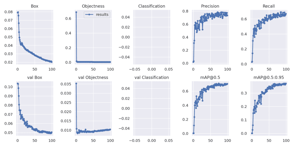
Results after training the YOLOv7 model using fixed-resolution images.
Now, let’s check the results of the test set.
!python test.py --weights runs/train/yolov7_pothole_fixed_res/weights/best.pt --task test --data data/pothole.yaml
Class      Images      Labels           P           R      mAP@.5  mAP@.5:.95: 100% 4/4 [00:05<00:00,  1.36s/it]
                all         118         304       0.725       0.684       0.686       0.395
We are getting much higher precision values on the test dataset also when training the larger model.
3.4 YOLOv7 Multi-Resolution Training
For the final training experiment, we will train the YOLOv7 model with multi-resolution images. For this case, we just need to add the –multi-scale flag and change the project name.
!python train.py --epochs 100 --workers 4 --device 0 --batch-size 8 --data data/pothole.yaml \
--img 640 640 --cfg cfg/training/yolov7_pothole.yaml --weights 'yolov7_training.pt' \
--name yolov7_pothole_multi_res --hyp data/hyp.scratch.custom.yaml \
--multi-scale
Epoch   gpu_mem       box       obj       cls     total    labels  img_size
    99/99     12.4G   0.02644   0.00577         0   0.03221        36       576: 100% 158/158 [01:40<00:00,  1.57it/s]
              Class      Images      Labels           P           R      mAP@.5  mAP@.5:.95: 100% 26/26 [00:10<00:00,  2.39it/s]
                all         401        1034       0.753       0.645       0.708       0.369
The results seem almost the same as the fixed resolution training with slightly higher mAP at 0.5 IoU.
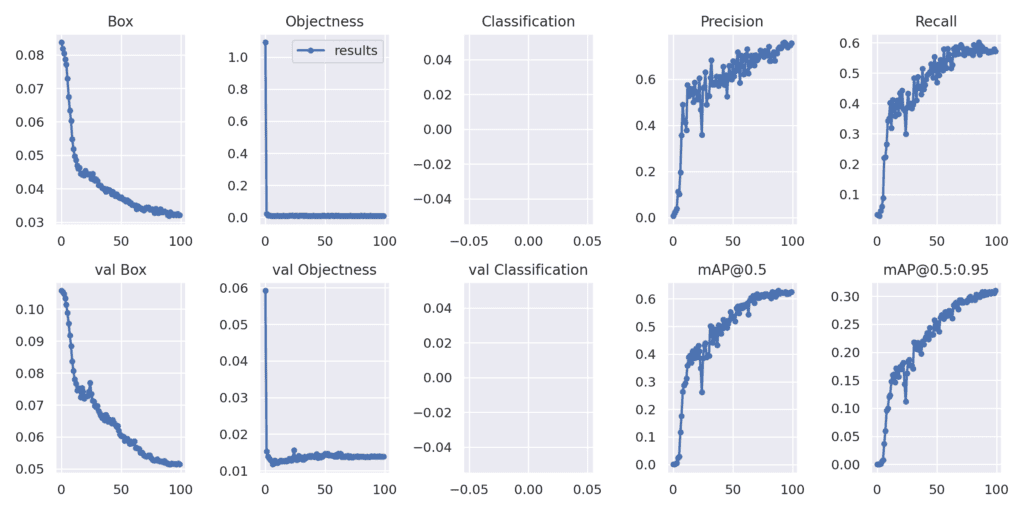
Results after training the YOLOv7 model using multi-resolution images.
The following block is for running the test using the latest multi-resolution trained model.
!python test.py --weights runs/train/yolov7_pothole_multi_res/weights/best.pt --task test --data data/pothole.yaml
The following are the results.
Class      Images      Labels           P           R      mAP@.5  mAP@.5:.95: 100% 4/4 [00:04<00:00,  1.22s/it]
                all         118         304       0.757       0.615       0.685       0.395
The results here look almost the same as the fixed-resolution model. But we can expect the multi-resolution training to perform better if we train for more epochs.
4. Running Inference using the Trained Models
We have four trained models with us. Let’s run inferences on videos using these and check out the results. For running the inference, we have copied the trained models along with their respective folders into the cloned yolov7 directory. We will run inference and check the outputs for each of the trained models here.
Do you want to know how YOLOv4 performs on the pothole detection dataset? Check out this post where we carry out pothole detection using YOLOv4 and Darknet.
4.1 Video Inference
Note: All inference experiments were run on a GTX 1060 6GB laptop GPU.
You may use the same command to run inference on videos of your choice by changing the video path.
Inference using the YOLOv7-Tiny Models
We have a sample video on which we can run inference using the following command. Let’s check out using the fixed-resolution trained model first.
python detect.py --source ../../inference_data/video.mp4 --weights runs/train/yolov7_tiny_pothole_fixed_res/weights/best.pt --view-img
And the following command can be used to run inference using the multi-resolution trained model.
python detect.py --source ../../inference_data/video.mp4 --weights runs/train/yolov7_tiny_pothole_multi_res/weights/best.pt --view-img
The following is the output.
The top part shows the output of the fixed-resolution tiny model and the bottom one for the multi-resolution model.
The fixed-resolution tiny model is performing well. But we can see a lot of fluctuations in the detections here. This can be due to less confident detections.
The detections with the multi-resolution trained model remain almost the same. But we can see that it can detect a few potholes that are farther away in a few cases compared to the fixed resolution trained model.
Inference using the YOLOv7 Models
Now, let’s check out the YOLOv7 trained models’ (large model) inference results. Beginning with the fixed-resolution trained model.
python detect.py --source ../../inference_data/video.mp4 --weights runs/train/yolov7_pothole_fixed_res/weights/best.pt --view-img
The next command is for the multi-resolution trained model inference.
python detect.py --source ../../inference_data/video.mp4 --weights runs/train/yolov7_pothole_multi_res/weights/best.pt --view-img
These results look much better. The potholes which far away have more confident detections with fewer fluctuations in the case of the YOLOv7 fixed resolution trained model.
The model trained with multi-resolution images has the best results in some of the cases. It is able to detect potholes that are much further away. But we can also see a few of the failure cases (false positives) where the model is detecting the lane markings as potholes. As it was trained on multi-resolution images, perhaps training this model even more will give the best results.
More Inference Comparison
Most of the time, when training with multi-resolution images, we may need to train for longer to get good results. This is necessary as the dataset becomes considerably difficult due to the varying image sizes. Also, the model gets to learn more images due to the varying features.
For that reason, in this section, we have inference results for a fixed-resolution model which has been trained for 100 epochs, and another multi-resolution trained model which has been trained for 275 epochs. The detection results have been overlaid on each other for easier comparison.
The orange bounding boxes represent the detections from the fixed-resolution 100 epochs training. And the green bounding boxes are from the multi-resolution 275 epochs training. Both of them are the YOLOv7 models.
On the one hand, it’s pretty clear that the model trained with fixed-resolution images is detecting the potholes which are slightly further away. But it has more false positives also. On the other hand, the model trained with fixed-resolution images is detecting more potholes, has much fewer false positives, and also the detected boxes are more bounded around the potholes.
There is going to be a tradeoff between training and getting the best out of fixed-resolution-trained models and multi-resolution-trained models. It is mostly based on the use case and the dataset. Even more important is running multiple experiments to find out which training settings and models work best.
4.2 FPS Comparison
The following is a graph showing the FPS and inference time (in milliseconds) comparisons between the different models which we ran the inferences for in the previous section.
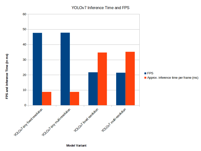
Graph showing the comparison between FPS and inference time for different YOLOv7 models.
You may get different FPS and inference time results depending on the hardware that you use for inference. Still, the YOLOv7-tiny models are going to be the fastest irrespective of whether they were trained on fixed or multi-resolution images.
5. Conclusion
We covered a lot in this blog post for fine tuning a YOLOv7 model. We chose a custom pothole detection dataset which was pretty challenging. Then we trained YOLOv7 and YOLOv7-tiny models with fixed and multi-resolution images. We also ran inference using the trained models to gain insight into the real-word inference results when using the models. We got to know which models are performing better compared to the others.
Hopefully, this blog post provided you with a lot of insights and ideas to carry out your own YOLOv7 fine tuning experiments. Do share in the comment section if you happen to get some interesting results.
Must Read Articles
Here are a few similar blog posts that you may be interested in.
- YOLOv7 Object Detection Paper Explanation and Inference
- Fine Tuning YOLOv7 on Custom Dataset
- YOLOv7 Pose vs MediaPipe in Human Pose Estimation
- YOLOv6 Object Detection – Paper Explanation and Inference
- YOLOX Object Detector Paper Explanation and Custom Training
- Object Detection using YOLOv5 and OpenCV DNN in C++ and Python
- Custom Object Detection Training using YOLOv5
- Pothole Detection using YOLOv4 and Darknet



100K+ Learners
Join Free OpenCV Bootcamp3 Hours of Learning