In this post, we will discuss the paper “EfficientNet: Rethinking Model Scaling for Convolutional Neural Networks”
At the heart of many computer vision tasks like image classification, object detection, segmentation, etc. is a Convolutional Neural Network (CNN).
In 2012, AlexNet won the ImageNet Large Scale Visual Recognition Competition (ILSVRC), beating the nearest competitor by nearly 10% in top-5 accuracy on ImageNet dataset.
AlexNet used a whopping 62 million parameters!
Soon people figured out the obvious ways in which AlexNet was not efficient. GoogleNet, the winner of ILSVRC 2014, used only 6.8 million parameters while being substantially more accurate than AlexNet.
After these initial inefficiencies were recognized and fixed, accuracy improvements in subsequent years came at the expense of an increased number of model parameters.
The table below shows the trend.
| Architecture | Year | Accuracy | Parameters |
|---|---|---|---|
| AlexNet | 2012 | 56.55% | 62M |
| GoogleNet | 2014 | 74.8% | 6.8M |
| SENet | 2017 | 82.7% | 145M |
| GPipe | 2018 | 84.3% | 557M |
Model Accuracy vs. Model Size Trade-off
Looking at the above table, we can see a trade-off between model accuracy and model size.
Even though we can notice a trade-off, it is not obvious how to design a new network that allows us to use this information. For example, we know GoogleNet has 6.8M parameters. How do we now design a network that is, say, half the size even though it is less accurate?
Here are a few options
- Model Compression: In this class of techniques, the original model is modified in a few clever ways like
- Pruning — Parameters that do not help accuracy are removed in a systematic way.
- Quantization — Model parameters are often stored as 32-bit floating point numbers, but these values are usually not uniformly distributed over the 32-bit space. Model quantization techniques examine the distribution of parameters and store the 32-bit numbers in a smaller number of bits without much loss of precision.
- Hand-crafting new networks: Often smaller networks are designed from scratch. SqueezeNets, MobileNets, and ShuffleNets are prime examples of networks designed with a smaller footprint in mind.
- Network Search: Another class of methods that is gaining popularity is an automated search for finding the best network depth, width, size of convolution kernels, etc. MnasNet is an example of this approach.
- Model Scaling: The final option is to use a standard network like GoogleNet or ResNet and scale it up (i.e. use larger parameters) or down (i.e. use fewer parameters) by changing the network’s depth and/or width, or the size of the input image. In this post, we will focus on Model Scaling because this is how EfficientNet achieves amazing performance.
Model Scaling
The idea of model scaling is to use a standard model like GoogleNet or ResNet and modify the architecture in one or more of the following ways.
- Change model depth: A CNN consists of several convolutional layers. These layers learn and encode different levels of abstraction of the input image. A CNN with a larger number of layers ( i.e. a deeper network ) can hold richer details about the image and is usually more accurate than a model with fewer layers ( i.e. a shallow network). E.g. ResNet-18 and ResNet-200 are both based on the ResNet architecture, but ResNet-200 is much deeper than ResNet-18 and is, therefore, more accurate. On the other hand, ResNet-18 is smaller and faster to run.
There are a few problems with using very deep networks- They are difficult to train due to the vanishing gradient problem.
- The gain in accuracy saturates after a certain depth.
- Change model width: A CNN layer also have multiple channels, much like the R, G, and B channels of an image. A network with more channels per layer is considered wider than a network with fewer channels. WideResNet and MobileNets are not very deep but are wide. These networks are easier to train, but they also suffer from the following problems.
- Extremely wide and shallow networks have difficulty capturing higher-level features.
- The gain in accuracy saturates after a certain width.
- Input image resolution: CNN architectures take in images of fixed size as input. It is obvious that a 512×512 image has more information than a 256×256 image. Therefore, one can change the architecture to take in a larger input image and improve accuracy. This increase in accuracy requires more processing power because a 512×512 image has 4x more pixels than a 256×256 image. Just as in the previous two cases, the gain in accuracy tends to saturate after a certain resolution.
The authors of the paper made the following two observations
- Scaling up any dimension of network width, depth, or resolution improves accuracy, but the accuracy gain diminishes for bigger models.
- To pursue better accuracy and efficiency, it is critical to balance all dimensions of network width, depth, and resolution during ConvNet scaling.
Both observations look intuitive.
What is not obvious is how to choose how much deeper or wider one should make the network or how much to increase the image size. Searching over one dimension, say depth, is itself very expensive. Searching over depth, width, and image resolution is almost impossible.
Compound Scaling
In the paper, the authors propose a compound scaling method that uses a compound coefficient of ![]() to uniformly scale width, depth, and resolution in a principled way
to uniformly scale width, depth, and resolution in a principled way
They propose the following formula
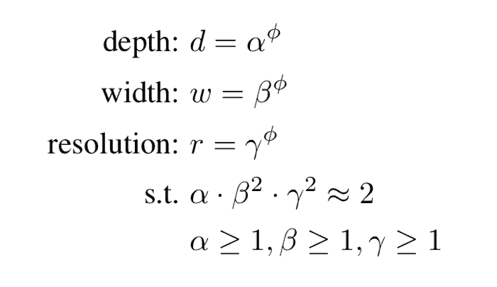
![]() is a user-specified coefficient that controls resources (e.g. Floating Point Operations (FLOPs)) available for model scaling.
is a user-specified coefficient that controls resources (e.g. Floating Point Operations (FLOPs)) available for model scaling.
![]() distribute the resources to depth, width, and resolution respectively.
distribute the resources to depth, width, and resolution respectively.
The FLOPS consumed in a convolutional operation is proportional to ![]() ,
, ![]() , and
, and ![]() , which is reflected in the above equation. The authors restrict
, which is reflected in the above equation. The authors restrict ![]() to 2 so that every new
to 2 so that every new ![]() , the FLOPs needed goes by up
, the FLOPs needed goes by up ![]()
What is EfficientNet-B0?
The above equation suggests we can do model scaling on any CNN architecture. While that is true, the authors found that the choice of the initial model to scale makes a difference in the final output.
So they developed their own baseline architecture and called it EfficientNet-B0. Like MnasNet, it was trained with a multi-objective neural architecture search that optimizes accuracy and FLOPS. So, the final architecture is similar to MnasNet.
The following table from the paper summarizes the architecture.
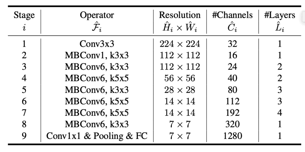
We have also linked to the detailed EfficientNet-B0 architecture here.
Model Scaling EfficientNet-B0
Starting with EfficientNet-B0, the authors used the following strategy to scale it up.
- Fix
 .
. - Assume the resource available at any step of scaling is twice of the resource at the previous step.
- Do a small grid search over
 ,
,  , and
, and  such that the constraint in the above equation is not violated.
 - The authors found the parameters
 = 1.2,
  =
=
1.1, = 1.15 to work the best.
 - Fix
 ,
,  , and
, and  as constants and scale up EfficientNet-B0 with different
  to obtain new scaled networks EfficientNet-B1 to B7.
You may wonder why ![]() ,
, ![]() , and
, and ![]() are not re-evaluated at every scaling step. The reason is that it is computationally expensive to do so.
are not re-evaluated at every scaling step. The reason is that it is computationally expensive to do so.
EfficientNet Performance
The graph below, taken from the paper, shows the performance curve of the EfficientNet family.
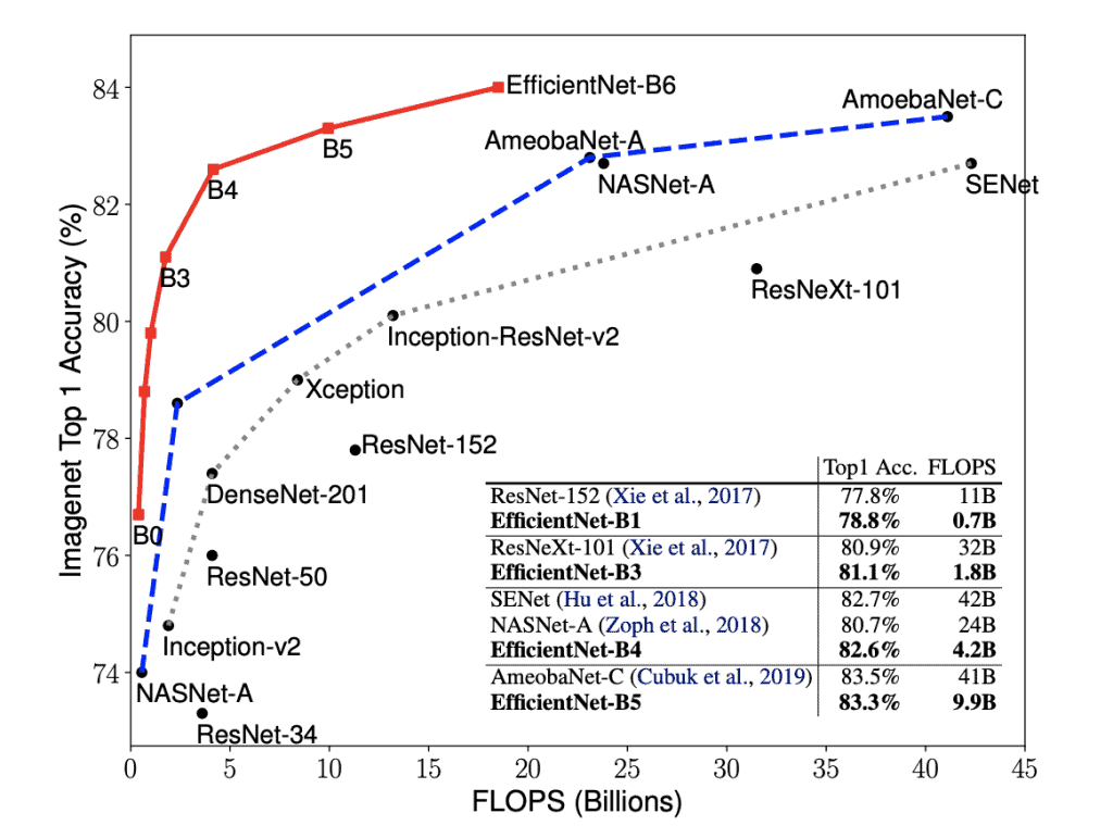
It shows that for the same FLOPS, the accuracy of EfficientNet than any existing architecture. So, if you plan to use Inception-v2, you should consider using EfficientNet-B1 instead. Similarly, it is a good idea to consider EfficientNet-B2 if you plan to use ResNet-50.
In most real-world applications, people start with a pre-trained model and fine-tune it for their specific application.
Just because EfficientNet outperforms other networks, does it mean it will outperform other networks on other tasks?
The good news is that the authors have done those experiments and shown that when the EfficientNet backbone is used, we also get better performance in other computer vision tasks.
EfficientNet Code in PyTorch & Keras
The authors have generously released pre-trained weights for EfficentNet-B0 – B5 for TensorFlow.
EfficientNet-B0 – B5 PyTorch models are also available.
All example code shared in this post has been written by my teammate Vishwesh Shrimali.
EfficientNet with PyTorch
First, let’s load the required modules.
# Load required modules
import json
from PIL import Image

import torch
from torchvision import transforms
We will use torch hub to load the pre-trained EfficientNet-B0 model.
# Load model from torch hub
model = torch.hub.load('rwightman/gen-efficientnet-pytorch', 'efficientnet_b0', pretrained=True)
Next, let’s open the image on which we want to perform model inference.
# Download the image
wget https://github.com/qubvel/efficientnet/raw/master/misc/panda.jpg
img = Image.open('panda.jpg')

Before we proceed with the next steps, let’s also download the labels file.
# Download labels file
wget https://raw.githubusercontent.com/lukemelas/EfficientNet-PyTorch/master/examples/simple/labels_map.txt
# Load class names
labels_map = json.load(open('labels_map.txt'))
labels_map = [labels_map[str(i)] for i in range(1000)]
Now, let’s pre-process the image before passing it to the model for inference.
# Preprocess image
tfms = transforms.Compose([transforms.Resize(image_size), transforms.CenterCrop(image_size),
                           transforms.ToTensor(),
                           transforms.Normalize([0.485, 0.456, 0.406], [0.229, 0.224, 0.225]),])
img = tfms(img).unsqueeze(0)

# Perform model inference
model.eval()
with torch.no_grad():
    logits = model(img)
preds = torch.topk(logits, k=5).indices.squeeze(0).tolist()

for idx in preds:
    label = labels_map[idx]
    prob = torch.softmax(logits, dim=1)[0, idx].item()
    print('{:<75} ({:.2f}%)'.format(label, prob*100))
Here is the output that you should get after running the above commands.
giant panda, panda, panda bear, coon bear, Ailuropoda melanoleuca           (90.13%)
ice bear, polar bear, Ursus Maritimus, Thalarctos maritimus                 (0.52%)
lesser panda, red panda, panda, bear cat, cat bear, Ailurus fulgens         (0.32%)
American black bear, black bear, Ursus americanus, Euarctos americanus      (0.10%)
soccer ball                                                                 (0.08%)
So, the model could predict that the image was of a Panda with 90% confidence.
Let’s try the same with Keras and see what kind of results we obtain.
EfficientNet with Keras
First, we will install efficientnet module, which will provide us with the EfficientNet-B0 pre-trained model that we will use for inference.
pip install efficientnet
Now, let’s load the required modules.
from keras.applications.imagenet_utils import decode_predictions
import numpy as np
import matplotlib.pyplot as plt
from efficientnet import EfficientNetB0
# Import image transformations
from efficientnet import center_crop_and_resize, preprocess_input
Let’s now load the pre-trained model.
model = EfficientNetB0(weights='imagenet')
We will use the same image as before for the model inference.
image = plt.imread('panda.jpg')
Finally, we will pre-process the image and pass it to the model for inference.
# preprocess input
image_size = model.input_shape[1]
x = center_crop_and_resize(image, image_size=image_size)
x = preprocess_input(x)
x = np.expand_dims(x, 0)

# make prediction and decode
y = model.predict(x)
decode_predictions(y)
Here is the output that you should get.
[[('n02510455', 'giant_panda', 0.8347929),
  ('n02134084', 'ice_bear', 0.0156020615),
  ('n02509815', 'lesser_panda', 0.004553518),
  ('n02133161', 'American_black_bear', 0.0024719085),
  ('n02132136', 'brown_bear', 0.002070759)]]
In this case, the model was able to predict that image was of a Giant Panda with an accuracy of 83.5%.






100K+ Learners
Join Free OpenCV Bootcamp3 Hours of Learning