An In-Depth Guide to Denoising Diffusion Probabilistic Models DDPM – Theory to Implementation

Diffusion probabilistic models are an exciting new area of research showing great promise in image generation. In retrospect, diffusion-based generative models were first introduced in 2015 and popularized in 2020 when Ho et al. published the paper “Denoising Diffusion Probabilistic Models” (DDPM). DDPMs are responsible for making diffusion models practical. In this article, we will highlight the key concepts and techniques behind DDPMs and train DDPMs from scratch on a “flowers” dataset for unconditional image generation.

In DDPMs, the authors changed the formulation and model training procedures which helped to improve and achieve “image fidelity” rivaling GANs and established the validity of these new generative algorithms.

The best approach to completely understanding “Denoising Diffusion Probabilistic Models”  is by going over both theory (+ some math) and the underlying code. With that in mind, let’s explore the learning path where:

• We’ll first explain what generative models are and why they are needed.
• We’ll discuss, from a theoretical standpoint, the approach used in diffusion-based generative models
• We’ll explore all the math necessary to understand denoising diffusion probabilistic models.
• Finally, we’ll discuss the training and inference used in DDPMs for image generation and code it from scratch in PyTorch. 

1. The Need For Generative Models
2. What Are Diffusion Probabilistic Models?
   1. Forward Diffusion Process
   2. Reverse Diffusion Process
3. Itsy-Bitsy Mathematical Details Behind Denoising Diffusion Probabilistic Models
   1. Mathematical Details Of The Forward Diffusion Process
   2. Mathematical Details Of The Reverse Diffusion Process
   3. Training Objective & Loss Function Used In Denoising Diffusion Probabilistic Models
4. Writing DDPMs From Scratch In PyTorch
5. Creating PyTorch Dataset Class Object
6. Creating PyTorch Dataloader Class Object
7. Visualizing Dataset
8. Model Architecture Used In DDPMs
9. Diffusion Class
10. Python Code For Forward Diffusion Process
11. Training & Sampling Algorithms Used In Denoising Diffusion Probabilistic Models
12. Training DDPMs From Scratch
13. Generating images using DDPMs
14. Summary

The Need For Generative Models

The job of image-based generative models is to generate new images that are similar, in other words, “representative” of our original set of images.

We need to create and train generative models because the set of all possible images that can be represented by, say, just (256x256x3) images is enormous. An image must have the right pixel value combinations to represent something meaningful (something we can understand).

For example, for the above image to represent a “Sunflower”, the pixels in the image need to be in the right configuration (they need to have the right values). And the space where such images exist is just a fraction of the entire set of images that can be represented by a (256x256x3) image space.

Now, if we knew how to get/sample a point from this subspace, we wouldn’t need to build “‘generative models.”  However, at this point in time, we don’t. 😓

The probability distribution function or, more precisely, probability density function (PDF) that captures/models this (data) subspace remains unknown and most likely too complex to make sense.

This is why we need ‘Generative models — To figure out the underlying likelihood function our data satisfies.

PS: A PDF is a “probability function” representing the density (likelihood) of a continuous random variable – which, in this case, means a function representing the likelihood of an image lying between a specific range of values defined by the function’s parameters. 

PPS: Every PDF has a set of parameters that determine the shape and probabilities of the distribution. The shape of the distribution changes as the parameter values change. For example, in the case of a normal distribution, we have mean µ (mu) and variance σ² (sigma) that control the distribution’s center point and spread.

What Are Diffusion Probabilistic Models?

In our previous post, “Introduction to Diffusion Models for Image Generation”, we didn’t discuss the math behind these models. We provided only a conceptual overview of how diffusion models work and focused on different well-known models and their applications. In this article, we’ll be focusing heavily on the first part.

In this section, we’ll explain diffusion-based generative models from a logical and theoretical perspective. Next, we’ll review all the math required to understand and implement Denoising Diffusion Probabilistic Models from scratch.

Diffusion models are a class of generative models inspired by an idea in Non-Equilibrium Statistical Physics, which states:

“We can gradually convert one distribution into another using a Markov chain”

– Deep Unsupervised Learning using Nonequilibrium Thermodynamics, 2015

Diffusion generative models are composed of two opposite processes i.e., Forward & Reverse Diffusion Process.

Forward Diffusion Process:

“It’s easy to destroy but hard to create”

– Pearl S. Buck

1. In the “Forward Diffusion” process, we slowly and iteratively add noise to (corrupt) the images in our training set such that they “move out or move away” from their existing subspace.
2. What we are doing here is converting the unknown and complex distribution that our training set belongs to into one that is easy for us to sample a (data) point from and understand.
3. At the end of the forward process, the images become entirely unrecognizable. The complex data distribution is wholly transformed into a (chosen) simple distribution. Each image gets mapped to a space outside the data subspace.

Reverse Diffusion Process:

By decomposing the image formation process into a sequential application of denoising autoencoders, diffusion models (DMs) achieve state-of-the-art synthesis results on image data and beyond.

Stable Diffusion, 2022

1. In the “Reverse Diffusion process,” the idea is to reverse the forward diffusion process.
2. We slowly and iteratively try to reverse the corruption performed on images in the forward process.
3. The reverse process starts where the forward process ends.
4. The benefit of starting from a simple space is that we know how to get/sample a point from this simple distribution (think of it as any point outside the data subspace). 
5. And our goal here is to figure out how to return to the data subspace.
6. However, the problem is that we can take infinite paths starting from a point in this “simple” space, but only a fraction of them will take us to the “data” subspace. 
7. In diffusion probabilistic models, this is done by referring to the small iterative steps taken during the forward diffusion process. 
8. The PDF that satisfies the corrupted images in the forward process differs slightly at each step.
9. Hence, in the reverse process, we use a deep-learning model at each step to predict the PDF parameters of the forward process. 
10. And once we train the model, we can start from any point in the simple space and use the model to iteratively take steps to lead us back to the data subspace. 
11. In reverse diffusion, we iteratively perform the “denoising” in small steps, starting from a noisy image.
12. This approach for training and generating new samples is much more stable than GANs and better than previous approaches like variational autoencoders (VAE) and normalizing flows. 

Since their introduction in 2020, DDPMs has been the foundation for cutting-edge image generation systems, including DALL-E 2, Imagen, Stable Diffusion, and Midjourney.

With the huge number of AI art generation tools today, it is difficult to find the right one for a particular use case. In our recent article, we explored all the different AI art generation tools so that you can make an informed choice to generate the best art.

Itsy-Bitsy Mathematical Details Behind Denoising Diffusion Probabilistic Models

As the motive behind this post is “creating and training Denoising Diffusion Probabilistic models from scratch,” we may have to introduce not all but some of the mathematical magic behind them.

In this section, we’ll cover all the required math while making sure it’s also easy to follow.

Let’s begin…

There are two terms mentioned on the arrows:

1. –
   1. This term is also known as the forward diffusion kernel (FDK).
   2. It defines the PDF of an image at timestep t in the forward diffusion process x_t given image x_t-1.
   3. It denotes the “transition function” applied at each step in the forward diffusion process. 
      
2. –
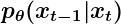
   1.  Similar to the forward process, it is known as the reverse diffusion kernel (RDK).
   2. It stands for the PDF of x_t-1 given x_t as parameterized by 𝜭. The 𝜭 means that the parameters of the distribution of the reverse process are learned using a neural network.
   3. It’s the “transition function” applied at each step in the reverse diffusion process. 

Mathematical Details Of The Forward Diffusion Process

The distribution q in the forward diffusion process is defined as Markov Chain given by:

1. We begin by taking an image from our dataset: x₀. Mathematically it’s stated as sampling a data point from the original (but unknown) data distribution: x₀ ~ q(x₀). 
2. The PDF of the forward process is the product of individual distribution starting from timestep 1 → T.  
3. The forward diffusion process is fixed and known.
4. All the intermediate noisy images starting from timestep 1 to T are also called “latents.” The dimension of the latents is the same as the original image.
5. The PDF used to define the FDK is a “Normal/Gaussian distribution” (eqn. 2).
6. At each timestep t, the parameters that define the distribution of image x_t are set  as:
   • Mean:
   • Covariance:
7. The term 𝝱 (beta) is known as the “diffusion rate” and is precalculated using a “variance scheduler”. The term I is an identity matrix. Therefore, the distribution at each time step is called Isotropic Gaussian. 
8. The original image is corrupted at each time step by adding a small amount of gaussian noise (ɛ). The amount of noise added is regulated by the scheduler.
9. By choosing sufficiently large timesteps and defining a well-behaved schedule of 𝝱_t the repeated application of FDK gradually converts the data distribution to be nearly an isotropic gaussian distribution.

How do we get image x_t from x_t-1 and how is noise added at each time step?

This can be easily understood by using the reparameterization trick in variational autoencoders.

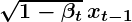
Referring to the second equation, we can easily sample image x_t from a normal distribution as:

1. Here, the epsilon ɛ is the “noise” term that is randomly sampled from the standard gaussian distribution and is first scaled and then added (scaled) x_(t-1).
2. In this way, starting from x₀, the original image is iteratively corrupted from t=1…T

In practice, the authors of DDPMs use a “linear variance scheduler” and define 𝝱 in the range [0.0001, 0.02] and set the total timesteps T = 1000 

“Diffusion models scale down the data with each forward process step (by a factor) so that variance does not grow when adding noise.“

– Denoising Diffusion Probabilistic Models, 2020

There’s a problem here, which results in an inefficient forward process 🐢.

Whenever we need a latent sample x at timestep t, we have to perform t-1 steps in the Markov chain.

To fix this, the authors of the DDPM reformulated the kernel to directly go from timestep 0 (i.e., from the original image) to timestep t in the process.

To do so, two additional terms are defined:

where eqn. (5) is a cumulative product of 𝛂 from 1 to t.

And then, by substituting 𝝱’swith 𝛂’sand using the addition property of Gaussian distribution. The forward diffusion process can be rewritten in terms of 𝛂 as:

🚀 Using the above formulation, we can sample at any arbitrary timestep t in the Markov chain.

That’s all for the forward diffusion process.

Mathematical Details Of The Reverse Diffusion Process

“In the reverse diffusion process, the task is to learn a finite-time (within T timesteps) reversal of the forward diffusion process.”

This basically means that we have to “undo” the forward process i.e., to remove the noise added in the forward process iteratively. It is done using a neural network model.

In the forward process, the transitions function q was defined using a Gaussian, so what function should be used for the reverse process p? What should the neural network learn? 

1. In 1949, W. Feller showed that, for gaussian (and binomial) distributions, the diffusion process’s reversal has the same functional form as the forward process.
2. This means that similar to the FDK, which is defined as a normal distribution, we can use the same functional form (a gaussian distribution) to define the reverse diffusion kernel. 
3. The reverse process is also a Markov chain where a neural network predicts the parameters for the reverse diffusion kernel at each timestep. 
4. During training, the learned estimates (of the parameters) should be close to the parameters of the FDK’s posterior at each timestep. We’ll talk more about FDK’s posterior in the next section.
5. We want this because if we follow the forward trajectory in reverse, we may return to the original data distribution.
6. In doing so, we would also learn how to generate new samples that closely match the underlying data distribution, starting from a pure gaussian noise (we do not have access to the forward process during inference).

1. The Markov chain for the reverse diffusion starts from where the forward process ends, i.e., at timestep T, where the data distribution has been converted into (nearly an) isotropic gaussian distribution.

      

      

      

2. The PDF of the reverse diffusion process is an “integral” over all the possible pathways we can take to arrive at a data sample (in the same distribution as the original) starting from pure noise x_T.

      

      

Training Objective & Loss Function Used In Denoising Diffusion Probabilistic Models

The training objective of diffusion-based generative models amounts to “maximizing the log-likelihood of the sample generated (at the end of the reverse process) (x) belonging to the original data distribution.”

We have defined the transition functions in diffusion models as “Gaussians”. To maximize the log-likelihood of a gaussian distribution, it is to try and find the parameters of the distribution (𝞵_, 𝝈²) such that it maximizes the “likelihood” of the (generated) data belonging to the same data distribution as the original data.

To train our neural network, we define the loss function (L) as the objective function’s negative. So a high value for p_𝜭(x₀), means low loss and vice versa.

Turns out, this is intractable because we need to integrate over a very high dimensional (pixel) space for continuous values over T timesteps.

Instead, the authors take inspiration from VAEs and reformulate the training objective using a variational lower bound (VLB), also known as “Evidence lower bound” (ELBO), which is this scary-looking equation 👻:

After some simplification, the DDPM authors arrive at this final L_vlb– Variational Lower Bound loss term:

We can break the above L_vlb loss term into individual timestep as follows:

You may notice that this loss function is huge! But the authors of DDPM further simplify it by ignoring some of the terms in their simplified loss function.

The terms ignored are:

1. L₀ – The authors got better results without this.
2. L_T – This is the “KL divergence” between the distribution of the final latent in the forward process and the first latent in the reverse process. However, there are no neural network parameters involved here, so we can’t do anything about it except define a good variance scheduler and use large timesteps such that they both represent an Isotropic Gaussian distribution.

So L_t-1 is the only loss term left which is a KL divergence between the “posterior” of the forward process (conditioned on x_t and the initial sample x₀), and the parameterized reverse diffusion process. Both terms are gaussian distributions as well.

The term q(x_t-1|x_t, x₀) is referred to as “forward process posterior distribution.” 

The job of our deep-learning model during training is to approximate/estimate the parameters of this (gaussian) posterior such that the KL divergence is as minimal as possible. 

The parameters of the posterior distribution are as follows:

To further simplify the task of the model, the authors decided to fix the variance to a constant 𝝱_t.

Now, the model only needs to learn to predict the above equation. And the reverse diffusion kernel gets modified to:

As we have kept the variance constant, minimizing KL divergence is as simple as minimizing the difference (or distance) between means (𝞵) of two gaussian distributions q and p (for e.g. difference between the means of distributions in the left image), which can be done as follows:

Now, there are three approaches we can take here:

1. Directly predict x₀ and find using it in the posterior function.
2. Predict the entire term.
3. Predict the noise at each timestep. This is done by writing the x₀ in in terms of x_t using the reparameterization trick.

By using the third option, and after some simplification, can be expressed as:

Similarly, the formulation for 𝞵_𝞱(x_t, t) is set to:

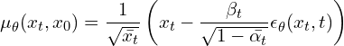
At training and inference time, we know the 𝝱’s, 𝛂’s, and x_t . So our model only needs to predict the noise at each timestep. The simplified (after ignoring some weighting terms) loss function used in the Denoising Diffusion Probabilistic Models is as follows:

Which is basically: 

This is the final loss function we use to train DDPMs, which is just a “Mean Squared Error” between the noise added in the forward process and the noise predicted by the model. This is the most impactful contribution of the paper Denoising Diffusion Probabilistic Models.

It’s awesome because, beginning from those scary-looking ELBO terms, we ended up with the simplest loss function in the entire machine learning domain.

Introduced in 2014 by Ian Goodfellow, Generative Adversarial Networks (GANs) were the norm for generating image samples. 

Many variations from the original GANs were created, such as:

1. Conditional GAN (cGAN): Controlling the class/category of the generated images.
2. Deep Convolutional GAN (DCGAN):  architecture significantly improves the quality of GANs using convolutional layers. 
3. Image-to-Image translation with Pix2Pix: Converting images from one domain to another by learning a mapping between the input and output.

Writing DDPMs From Scratch In PyTorch

From this section, we’ll code all the essential components required for training denoising diffusion probabilistic models from scratch in PyTorch. Instead of Colab, we used Kaggle kernels as it provides better GPUs than Colab free version and longer training times (which is crucial for diffusion models).

Note: code for regularly used helper functions is not added to the post.

💡 You can access the entire codebase for this and all our other posts by simply subscribing to the blog post, and we’ll send you the link to download link.

Click here to download the source code to this post

First and foremost, we’ll define configuration classes that will hold the hyperparameters for loading the dataset, creating log directories, and training the model.

from dataclasses import dataclass

@dataclass
class BaseConfig:
    DEVICE = get_default_device()
    DATASET = "Flowers"  #  "MNIST", "Cifar-10", "Flowers"

    # For logging inferece images and saving checkpoints.
    root_log_dir = os.path.join("Logs_Checkpoints", "Inference")
    root_checkpoint_dir = os.path.join("Logs_Checkpoints", "checkpoints")

    # Current log and checkpoint directory.
    log_dir = "version_0"
    checkpoint_dir = "version_0"


@dataclass
class TrainingConfig:
    TIMESTEPS = 1000  # Define number of diffusion timesteps
    IMG_SHAPE = (1, 32, 32) if BaseConfig.DATASET == "MNIST" else (3, 32, 32)
    NUM_EPOCHS = 800
    BATCH_SIZE = 32
    LR = 2e-4
    NUM_WORKERS = 2

Creating PyTorch Dataset Class Object

This article uses the “Flowers” dataset, which can be downloaded from Kaggle or quickly loaded in the Kaggle kernel environment. But as you may have noticed, in the BaseConfig class, we have also provided the option to load the MNIST, Cifar-10 and Cifar-100 datasets. You can choose whichever one you prefer. 

The flowers dataset can be downloaded from over here: Flowers Recognition | Kaggle

When using Kaggle kernels, it’s as simple as just clicking on the “Add Data” component and selecting the dataset.

Here, we are creating two functions:

1. get_dataset(...): Returns the dataset class object that will be passed to the Dataloader. Three preprocessing transforms, and one augmentation are applied to every image in the dataset.
   1. Preprocessing:
      1. Convert pixel values from the range [0, 255] → [0.0, 1.0]
      2. Resize Images to shape (32x32).
      3. Change pixel values from the range [0.0, 1.0] → [-1.0, 1.0]. This is done by the DDPM authors so that the input image roughly has the same range of values as a standard gaussian.
   2. Augmentation:
      1. A random horizontal flip, as used in the original implementation. In case you are using the MNIST dataset, be sure to comment out this line.
2. inverse_transforms(...): This function is used for inverting the transforms applied during the loading step and reverting the image to the range [0.0, 255.0].

import torchvision
import torchvision.transforms as TF
import torchvision.datasets as datasets
from torch.utils.data import Dataset, DataLoader


def get_dataset(dataset_name='MNIST'):
    transforms = torchvision.transforms.Compose(
        [
            torchvision.transforms.ToTensor(),
            torchvision.transforms.Resize((32, 32), 
                                          interpolation=torchvision.transforms.InterpolationMode.BICUBIC, 
                                          antialias=True),
            torchvision.transforms.RandomHorizontalFlip(),
#             torchvision.transforms.Normalize(MEAN, STD),
            torchvision.transforms.Lambda(lambda t: (t * 2) - 1) # Scale between [-1, 1] 
        ]
    )
    
    if dataset_name.upper() == "MNIST":
        dataset = datasets.MNIST(root="data", train=True, download=True, transform=transforms)
    elif dataset_name == "Cifar-10":    
        dataset = datasets.CIFAR10(root="data", train=True, download=True, transform=transforms)
    elif dataset_name == "Cifar-100":
        dataset = datasets.CIFAR10(root="data", train=True, download=True, transform=transforms)
    elif dataset_name == "Flowers":
        dataset = datasets.ImageFolder(root="/kaggle/input/flowers-recognition/flowers", transform=transforms)

    return dataset

def inverse_transform(tensors):
    """Convert tensors from [-1., 1.] to [0., 255.]"""
    return ((tensors.clamp(-1, 1) + 1.0) / 2.0) * 255.0

Creating PyTorch Dataloader Class Object

Next, we define the get_dataloader(...) function that returns a Dataloader object for the chosen dataset.

def get_dataloader(dataset_name='MNIST', 
                   batch_size=32, 
                   pin_memory=False, 
                   shuffle=True, 
                   num_workers=0, 
                   device="cpu"
                  ):
    dataset      = get_dataset(dataset_name=dataset_name)
    dataloader = DataLoader(dataset, batch_size=batch_size, 
                            pin_memory=pin_memory, 
                            num_workers=num_workers, 
                            shuffle=shuffle
                           )
    # Used for moving batch of data to the user-specified machine: cpu or gpu
    device_dataloader = DeviceDataLoader(dataloader, device)
    return device_dataloader

Visualizing Dataset

First, we’ll create the “dataloader” object by calling the get_dataloader(...) function.

loader = get_dataloader(
    dataset_name=BaseConfig.DATASET,
    batch_size=128,
    device=”cpu”,
)

Then we can simply use torchvision’s make_grid(...) function to plot a grid of flower images.

from torchvision.utils import make_grid

plt.figure(figsize=(10, 4), facecolor='white')

for b_image, _ in loader:
    b_image = inverse_transform(b_image)
    grid_img = make_grid(b_image / 255.0, nrow=16, padding=True, pad_value=1)
    plt.imshow(grid_img.permute(1, 2, 0))
    plt.axis("off")
    break

Model Architecture Used In DDPMs

In DDPMs, the authors use a UNet-shaped deep neural network which takes in as input:

1. The input image at any stage of the reverse process.
2. The timestep of the input image.

From the usual UNet architecture, the authors replaced the original double convolution at each level with “Residual blocks” used in ResNet models.

The architecture comprises 5 components:

1. Encoder blocks
2. Bottleneck blocks
3. Decoder blocks
4. Self attention modules
5. Sinusoidal time embeddings

Architectural Details:

1. There are four levels in the encoder and decoder path with bottleneck blocks between them.
2. Each encoder stage comprises two residual blocks with convolutional downsampling except the last level.
3. Each corresponding decoder stage comprises three residual blocks and uses 2x nearest neighbors with convolutions to upsample the input from the previous level.
4. Each stage in the encoder path is connected to the decoder path with the help of skip connections. 
5. The model uses “Self-Attention” modules at a single feature map resolution. 
6. Every residual block in the model gets the inputs from the previous layer (and others in the decoder path) and the embedding of the current timestep. The timestep embedding informs the model of the input’s current position in the Markov chain.

In this article, we are working on an image size of (32×32). Only two minor changes exist between our model and the original model used in the paper. 

1. We use 64 base channels instead of 128.
2. There are four levels in both encoder and decoder paths. The feature maps size at each level are kept as follows: 32 →16 → 8 → 8. We are applying self-attention at feature map sizes of both (16x16) and (8x8) as opposed to the original, where they are applied just once at a feature map size of (16x16).

Please note that we are not adding the model code because the code for the UNet + these modifications is quite easy, but because of all the different components. it becomes just too big to be added to the post.

Diffusion Class

In this section, we are creating a class called SimpleDiffusion. This class contains:

1. Scheduler constants required for performing the forward and reverse diffusion process.
2. A method to define the linear variance scheduler used in DDPMs.
3. A method that performs a single step using the updated forward diffusion kernel.

class SimpleDiffusion:
    def __init__(
        self,
        num_diffusion_timesteps=1000,
        img_shape=(3, 64, 64),
        device="cpu",
    ):
        self.num_diffusion_timesteps = num_diffusion_timesteps
        self.img_shape = img_shape
        self.device = device
        self.initialize()

    def initialize(self):
        # BETAs & ALPHAs required at different places in the Algorithm.
        self.beta  = self.get_betas()
        self.alpha = 1 - self.beta
        
        self_sqrt_beta                       = torch.sqrt(self.beta)
        self.alpha_cumulative                = torch.cumprod(self.alpha, dim=0)
        self.sqrt_alpha_cumulative           = torch.sqrt(self.alpha_cumulative)
        self.one_by_sqrt_alpha               = 1. / torch.sqrt(self.alpha)
        self.sqrt_one_minus_alpha_cumulative = torch.sqrt(1 - self.alpha_cumulative)
         
    def get_betas(self):
        """linear schedule, proposed in original ddpm paper"""
        scale = 1000 / self.num_diffusion_timesteps
        beta_start = scale * 1e-4
        beta_end = scale * 0.02
        return torch.linspace(
            beta_start,
            beta_end,
            self.num_diffusion_timesteps,
            dtype=torch.float32,
            device=self.device,
        )

Python Code For Forward Diffusion Process

In this section, we are writing the python code to perform the “forward diffusion process” in a single step as per the equation mentioned here.

The forward_diffusion(...) function takes in a batch of images and corresponding timesteps and adds noise/corrupts the input images using the updated forward diffusion kernel equation.

def forward_diffusion(sd: SimpleDiffusion, x0: torch.Tensor, timesteps: torch.Tensor):
    eps = torch.randn_like(x0)  # Noise
    mean    = get(sd.sqrt_alpha_cumulative, t=timesteps) * x0  # Image scaled
    std_dev = get(sd.sqrt_one_minus_alpha_cumulative, t=timesteps) # Noise scaled
    sample  = mean + std_dev * eps # scaled inputs * scaled noise

    return sample, eps  # return ... , gt noise --> model predicts this

Visualizing Forward Diffusion Process On Sample Images

In this section, we’ll visualize the forward diffusion process on some sample images to see how they get corrupted as they pass through the Markov chain for T timesteps.

sd = SimpleDiffusion(num_diffusion_timesteps=TrainingConfig.TIMESTEPS, device="cpu")

loader = iter(  # converting dataloader into an iterator for now.
    get_dataloader(
        dataset_name=BaseConfig.DATASET,
        batch_size=6,
        device="cpu",
    )
)

Performing the forward process for some specific timesteps and also storing the noisy versions of the original image.

x0s, _ = next(loader)

noisy_images = []
specific_timesteps = [0, 10, 50, 100, 150, 200, 250, 300, 400, 600, 800, 999]

for timestep in specific_timesteps:
    timestep = torch.as_tensor(timestep, dtype=torch.long)

    xts, _ = sd.forward_diffusion(x0s, timestep)
    xts    = inverse_transform(xts) / 255.0
    xts    = make_grid(xts, nrow=1, padding=1)
    
    noisy_images.append(xts)

Plotting sample corruption at different timesteps.

_, ax = plt.subplots(1, len(noisy_images), figsize=(10, 5), facecolor='white')

for i, (timestep, noisy_sample) in enumerate(zip(specific_timesteps, noisy_images)):
    ax[i].imshow(noisy_sample.squeeze(0).permute(1, 2, 0))
    ax[i].set_title(f"t={timestep}", fontsize=8)
    ax[i].axis("off")
    ax[i].grid(False)

plt.suptitle("Forward Diffusion Process", y=0.9)
plt.axis("off")
plt.show()

Training & Sampling Algorithms Used In Denoising Diffusion Probabilistic Models

Training code based on Algorithm 1: 

The first function defined here is train_one_epoch(...). This function is used for performing “one epoch of training ” i.e., it trains the model by iterating once over the entire dataset and will be called in our final training loop.

We also use Mixed-Precision training to train the model faster and save GPU memory. The code is pretty straightforward and almost a one-to-one conversion from the algorithm.

# Algorithm 1: Training

def train_one_epoch(model, loader, sd, optimizer, scaler, loss_fn, epoch=800, 
                   base_config=BaseConfig(), training_config=TrainingConfig()):
    
    loss_record = MeanMetric()
    model.train()

    with tqdm(total=len(loader), dynamic_ncols=True) as tq:
        tq.set_description(f"Train :: Epoch: {epoch}/{training_config.NUM_EPOCHS}")
         
        for x0s, _ in loader: # line 1, 2
            tq.update(1)
            
            ts = torch.randint(low=1, high=training_config.TIMESTEPS, size=(x0s.shape[0],), device=base_config.DEVICE) # line 3
            xts, gt_noise = sd.forward_diffusion(x0s, ts) # line 4

            with amp.autocast():
                pred_noise = model(xts, ts)
                loss = loss_fn(gt_noise, pred_noise) # line 5

            optimizer.zero_grad(set_to_none=True)
            scaler.scale(loss).backward()

            # scaler.unscale_(optimizer)
            # torch.nn.utils.clip_grad_norm_(model.parameters(), 1.0)

            scaler.step(optimizer)
            scaler.update()

            loss_value = loss.detach().item()
            loss_record.update(loss_value)

            tq.set_postfix_str(s=f"Loss: {loss_value:.4f}")

        mean_loss = loss_record.compute().item()
    
        tq.set_postfix_str(s=f"Epoch Loss: {mean_loss:.4f}")
    
    return mean_loss

Sampling or Inference code based on Algorithm 2:

The next function we define is reverse_diffusion(...) which is responsible for performing inference i.e., generating images using the reverse diffusion process. The function takes in a trained model and the diffusion class and can either generate a video showcasing the entire diffusion process or just the final generated image. 

# Algorithm 2: Sampling
    
@torch.no_grad()
def reverse_diffusion(model, sd, timesteps=1000, img_shape=(3, 64, 64), 
                      num_images=5, nrow=8, device="cpu", **kwargs):

    x = torch.randn((num_images, *img_shape), device=device)
    model.eval()

    if kwargs.get("generate_video", False):
        outs = []

    for time_step in tqdm(iterable=reversed(range(1, timesteps)), 
                          total=timesteps-1, dynamic_ncols=False, 
                          desc="Sampling :: ", position=0):

        ts = torch.ones(num_images, dtype=torch.long, device=device) * time_step
        z = torch.randn_like(x) if time_step > 1 else torch.zeros_like(x)

        predicted_noise = model(x, ts)

        beta_t                            = get(sd.beta, ts)
        one_by_sqrt_alpha_t               = get(sd.one_by_sqrt_alpha, ts)
        sqrt_one_minus_alpha_cumulative_t = get(sd.sqrt_one_minus_alpha_cumulative, ts) 

        x = (
            one_by_sqrt_alpha_t
            * (x - (beta_t / sqrt_one_minus_alpha_cumulative_t) * predicted_noise)
            + torch.sqrt(beta_t) * z
        )

        if kwargs.get("generate_video", False):
            x_inv = inverse_transform(x).type(torch.uint8)
            grid = make_grid(x_inv, nrow=nrow, pad_value=255.0).to("cpu")
            ndarr = torch.permute(grid, (1, 2, 0)).numpy()[:, :, ::-1]
            outs.append(ndarr)

    if kwargs.get("generate_video", False): # Generate and save video of the entire reverse process. 
        frames2vid(outs, kwargs['save_path'])
        display(Image.fromarray(outs[-1][:, :, ::-1])) # Display the image at the final timestep of the reverse process.
        return None

    else: # Display and save the image at the final timestep of the reverse process. 
        x = inverse_transform(x).type(torch.uint8)
        grid = make_grid(x, nrow=nrow, pad_value=255.0).to("cpu")
        pil_image = TF.functional.to_pil_image(grid)
        pil_image.save(kwargs['save_path'], format=save_path[-3:].upper())
        display(pil_image)
        return None

Training DDPMs From Scratch

In the previous sections, we have already defined all the necessary classes and functions required for training. All we have to do now is assemble them and start the training process. 

Before we begin training:

• We’ll first define all the model-related hyperparameters.
• Then initialize the UNet model,  AdamW optimizer, MSE loss function, and other necessary classes.

@dataclass
class ModelConfig:
    BASE_CH = 64  # 64, 128, 256, 256
    BASE_CH_MULT = (1, 2, 4, 4) # 32, 16, 8, 8 
    APPLY_ATTENTION = (False, True, True, False)
    DROPOUT_RATE = 0.1
    TIME_EMB_MULT = 4 # 128

model = UNet(
    input_channels          = TrainingConfig.IMG_SHAPE[0],
    output_channels         = TrainingConfig.IMG_SHAPE[0],
    base_channels           = ModelConfig.BASE_CH,
    base_channels_multiples = ModelConfig.BASE_CH_MULT,
    apply_attention         = ModelConfig.APPLY_ATTENTION,
    dropout_rate            = ModelConfig.DROPOUT_RATE,
    time_multiple           = ModelConfig.TIME_EMB_MULT,
)
model.to(BaseConfig.DEVICE)

optimizer = torch.optim.AdamW(model.parameters(), lr=TrainingConfig.LR) # Original → Adam

dataloader = get_dataloader(
    dataset_name  = BaseConfig.DATASET,
    batch_size    = TrainingConfig.BATCH_SIZE,
    device        = BaseConfig.DEVICE,
    pin_memory    = True,
    num_workers   = TrainingConfig.NUM_WORKERS,
)

loss_fn = nn.MSELoss()

sd = SimpleDiffusion(
    num_diffusion_timesteps = TrainingConfig.TIMESTEPS,
    img_shape               = TrainingConfig.IMG_SHAPE,
    device                  = BaseConfig.DEVICE,
)

scaler = amp.GradScaler() # For mixed-precision training.

Then we’ll initialize the logging and checkpoint directories to save intermediate sampling results and model parameters.

total_epochs = TrainingConfig.NUM_EPOCHS + 1
log_dir, checkpoint_dir = setup_log_directory(config=BaseConfig())
generate_video = False
ext = ".mp4" if generate_gif else ".png"

Finally, we can write our training loop. As we have divided all our code into simple, easy-to-debug functions and classes, all we have to do now is call them in the epochs training loop. Specifically, we need to call the “training” and “sampling” functions defined in the previous section in a loop.

for epoch in range(1, total_epochs):
    torch.cuda.empty_cache()
    gc.collect()
    
    # Algorithm 1: Training
    train_one_epoch(model, sd, dataloader, optimizer, scaler, loss_fn, epoch=epoch)

    if epoch % 20 == 0:
        save_path = os.path.join(log_dir, f"{epoch}{ext}")
        
        # Algorithm 2: Sampling
        reverse_diffusion(model, sd, timesteps=TrainingConfig.TIMESTEPS, 
                          num_images=32, generate_video=generate_video, save_path=save_path, 
                          img_shape=TrainingConfig.IMG_SHAPE, device=BaseConfig.DEVICE, nrow=4,
        )

        # clear_output()
        checkpoint_dict = {
            "opt": optimizer.state_dict(),
            "scaler": scaler.state_dict(),
            "model": model.state_dict()
        }
        torch.save(checkpoint_dict, os.path.join(checkpoint_dir, "ckpt.pt"))
        del checkpoint_dict

If all goes well, the training procedure should start and print the training logs similar to:

Generating Images Using DDPMs

You can let the training complete for 800 epochs or interrupt in between if you are satisfied with the samples generated at every 20 epochs. 
To perform the inference, we simply have to reload the saved model, and you can use the same or a different logging directory to save the results. You can re-initialize the SimpleDiffusion class as well, but it’s not necessary.

# Reloading model from saved checkpoint
model = UNet(
    input_channels          = TrainingConfig.IMG_SHAPE[0],
    output_channels         = TrainingConfig.IMG_SHAPE[0],
    base_channels           = ModelConfig.BASE_CH,
    base_channels_multiples = ModelConfig.BASE_CH_MULT,
    apply_attention         = ModelConfig.APPLY_ATTENTION,
    dropout_rate            = ModelConfig.DROPOUT_RATE,
    time_multiple           = ModelConfig.TIME_EMB_MULT,
)
model.load_state_dict(torch.load(os.path.join(checkpoint_dir, "ckpt.tar"), map_location='cpu')['model'])

model.to(BaseConfig.DEVICE)

sd = SimpleDiffusion(
    num_diffusion_timesteps = TrainingConfig.TIMESTEPS,
    img_shape               = TrainingConfig.IMG_SHAPE,
    device                  = BaseConfig.DEVICE,
)

log_dir = "inference_results"

The inference code is simply a call to the reverse_diffusion(...) function using the trained model.

generate_video = False # Set it to True for generating video of the entire reverse diffusion proces or False to for saving only the final generated image.

ext = ".mp4" if generate_video else ".png"
filename = f"{datetime.now().strftime('%Y%m%d-%H%M%S')}{ext}"

save_path = os.path.join(log_dir, filename)

reverse_diffusion(
    model,
    sd,
    num_images=256,
    generate_video=generate_video,
    save_path=save_path,
    timesteps=1000,
    img_shape=TrainingConfig.IMG_SHAPE,
    device=BaseConfig.DEVICE,
    nrow=32,
)
print(save_path)

Some of the results we got:

Summary

In conclusion, diffusion models represent a rapidly growing field with a wealth of exciting possibilities for the future. As research in this area continues to evolve, we can expect even more advanced techniques and applications to emerge. I encourage readers to share their thoughts and questions about this topic and to engage in conversations about the future of diffusion models.

To summarise this article📜, we covered a comprehensive list of related topics.

1. We began by providing an intuitive answer to the fundamental question of why we need generative models.
2. Then we continued the discussion to explain diffusion-based generative models from a logical and theoretical perspective.
3. After building the theoretical base, we introduced all the necessary mathematical equations derived for DDPMs one by one while also maintaining the flow so that it’s easy to grasp.
4. Finally, we concluded by explaining all the different pieces of code required for training DDPMs from scratch and performing inference. We also demonstrated the results we got from our experiments. 

References

1. What are Diffusion Models?
2. DDPMs from scratch
3. Diffusion Models | Paper Explanation | Math Explained
4. Paper – Deep Unsupervised Learning using Nonequilibrium Thermodynamics
5. Paper – Denoising Diffusion Probabilistic Models
6. Paper – Improved Denoising Diffusion Probabilistic Models
7. Paper – A Survey on Generative Diffusion Model
8. An introduction to Diffusion Probabilistic Models – Ayan Das
9. Denoising diffusion probabilistic models – Param Hanji

We would love to hear from you. Please feel free to ask questions in the comment section; we are more than happy to converse with you.

🌟Happy learning!