In this post, we will understand what is Yolov3 and learn how to use YOLOv3 — a state-of-the-art object detector — with OpenCV.
YOLOv3 is the latest variant of a popular object detection algorithm YOLO – You Only Look Once. The published model recognizes 80 different objects in images and videos, but most importantly, it is super fast and nearly as accurate as Single Shot MultiBox (SSD).
Starting with OpenCV 3.4.2, you can easily use YOLOv3 models in your own OpenCV application.
This post mainly focuses on inference, but you can also find our tutorial on training YOLOv3 model on your dataset.
YOLO Master Post – Every Model Explained
Don’t miss out on this comprehensive resource — Mastering All Yolo Models for a richer, more informed perspective on the YOLO series.
How does YOLO work?
We can think of an object detector as a combination of an object locator and an object recognizer.
Traditional computer vision approaches used a sliding window to look for objects at different locations and scales. Because this was such an expensive operation, the aspect ratio of the object was usually assumed to be fixed.
Early Deep Learning based object detection algorithms like the R-CNN and Fast R-CNN used a method called Selective Search to narrow down the number of bounding boxes that the algorithm had to test.
Another approach called Overfeat involved scanning the image at multiple scales using sliding windows-like mechanisms done convolutionally.
This was followed by Faster R-CNN, which used a Region Proposal Network (RPN) to identify bounding boxes that needed testing. By clever design, the features extracted for recognizing objects were also used by the RPN for proposing potential bounding boxes, thus saving a lot of computation.
YOLO, on the other hand, approaches the object detection problem in a completely different way. It forwards the whole image only once through the network. SSD is another object detection algorithm that forwards the image through a deep learning network, but YOLOv3 is much faster than SSD while achieving comparable accuracy. YOLOv3 gives faster than real-time results on a M40, TitanX or 1080 Ti GPUs.
Let’s see how YOLO detects the objects in a given image.
First, it divides the image into a 13×13 grid of cells. The size of these 169 cells varies depending on the input size. For a 416×416 input size that we used in our experiments, the cell size was 32×32. Each cell is then responsible for predicting the number of boxes in the image.
For each bounding box, the network also predicts the confidence that the bounding box actually encloses an object, and the probability of the enclosed object being a particular class.
Most of these bounding boxes are eliminated because their confidence is low or because they are enclosing the same object as another bounding box with a very high confidence score. This technique is called non-maximum suppression.
The authors of YOLOv3, Joseph Redmon and Ali Farhadi have made YOLOv3 faster and more accurate than their previous work YOLOv2. YOLOv3 handles multiple scales better. They have also improved the network by making it bigger and taking it towards residual networks by adding shortcut connections.
Why use OpenCV for YOLO?
Here are a few reasons you may want to use OpenCV for YOLO
- Easy integration with an OpenCV application: If your application already uses OpenCV and you want to use YOLOv3, you don’t have to worry about compiling and building the extra Darknet code.
- OpenCV CPU version is 9x faster: OpenCV’s CPU implementation of the DNN module is astonishingly fast. For example, Darknet, when used with OpenMP takes about 2 seconds on a CPU for inference on a single image. In contrast, OpenCV’s implementation runs in a mere 0.22 seconds! Check out table below.
- Python support: Darknet is written in C and does not officially support Python. In contrast, OpenCV does. There are python ports available for Darknet, though.
Speed Test for YOLOv3 on Darknet and OpenCV
The following table shows the performance of YOLOv3 on Darknet vs. OpenCV. The input size in all cases is 416×416. It is not surprising the GPU version of Darknet outperforms everything else. It is also not suprising that Darknet with OpenMP works much better than Darknet without OpenMP because OpenMP enables use of multiple processors.
What is indeed surprising is that OpenCV’s CPU implementation of DNN is 9x faster than Darknet with OpenML.
Note: We ran into problems using OpenCV’s GPU implementation of the DNN. The documentation indicates that it is tested only with Intel’s GPUs, so the code would switch you back to CPU, if you do not have an Intel GPU.
Object Detection using YOLOv3 in C++/Python
Let us now see how to use YOLOv3 in OpenCV to perform object detection.
Step 1 : Download the models
We will start by downloading the models using the script file getModels.sh from the command line.
sudo chmod a+x getModels.sh
./getModels.sh
This will download the yolov3.weights file (containing the pre-trained network’s weights), the yolov3.cfg file (containing the network configuration) and the coco.names file, which contains the 80 different class names used in the COCO dataset.
Step 2 : Initialize the parameters
The YOLOv3 algorithm generates bounding boxes as the predicted detection outputs. Every predicted box is associated with a confidence score. In the first stage, all the boxes below the confidence threshold parameter are ignored for further processing.
The rest of the boxes undergo non-maximum suppression, removing redundant, overlapping bounding boxes. Non-maximum suppression is controlled by a parameter nmsThreshold. You can try to change these values and see how the number of output predicted boxes changes.
Next, the default values for the input width (inpWidth) and height (inpHeight) for the network’s input image are set. We set each of them to 416 to compare our runs to the Darknet’s C code given by YOLOv3’s authors. You can change both of them to 320 to get faster results or 608 to get more accurate results.
Python
# Initialize the parameters
confThreshold = 0.5  #Confidence threshold
nmsThreshold = 0.4   #Non-maximum suppression threshold
inpWidth = 416       #Width of network's input image
inpHeight = 416      #Height of network's input image
C++
// Initialize the parameters
float confThreshold = 0.5; // Confidence threshold
float nmsThreshold = 0.4;  // Non-maximum suppression threshold
int inpWidth = 416;        // Width of network's input image
int inpHeight = 416;       // Height of network's input image
Step 3 : Load the model and classes
The file coco.names contains all the objects for which the model was trained. We read class names.
Next, we load the network, which has two parts —
- yolov3.weights : The pre-trained weights.
- yolov3.cfg : The configuration file.
We set the DNN backend to OpenCV here and the target to CPU. You could try setting the preferable target to cv.dnn.DNN_TARGET_OPENCL to run it on a GPU. But keep in mind that the current OpenCV version is tested only with Intel’s GPUs; it would automatically switch to CPU, if you do not have an Intel GPU.
Python
# Load names of classes
classesFile = "coco.names";
classes = None
with open(classesFile, 'rt') as f:
classes = f.read().rstrip('\n').split('\n')

# Give the configuration and weight files for the model and load the network using them.
modelConfiguration = "yolov3.cfg";
modelWeights = "yolov3.weights";

net = cv.dnn.readNetFromDarknet(modelConfiguration, modelWeights)
net.setPreferableBackend(cv.dnn.DNN_BACKEND_OPENCV)
net.setPreferableTarget(cv.dnn.DNN_TARGET_CPU)
C++
// Load names of classes
string classesFile = "coco.names";
ifstream ifs(classesFile.c_str());
string line;
while (getline(ifs, line)) classes.push_back(line);

// Give the configuration and weight files for the model
String modelConfiguration = "yolov3.cfg";
String modelWeights = "yolov3.weights";

// Load the network
Net net = readNetFromDarknet(modelConfiguration, modelWeights);
net.setPreferableBackend(DNN_BACKEND_OPENCV);
net.setPreferableTarget(DNN_TARGET_CPU);
Step 4 : Read the input
In this step, we read the image, video stream, or webcam. In addition, we also open the video writer to save the frames with detected output bounding boxes.
Python
outputFile = "yolo_out_py.avi"
if (args.image):
    # Open the image file
    if not os.path.isfile(args.image):
        print("Input image file ", args.image, " doesn't exist")
        sys.exit(1)
    cap = cv.VideoCapture(args.image)
    outputFile = args.image[:-4]+'_yolo_out_py.jpg'
elif (args.video):
    # Open the video file
    if not os.path.isfile(args.video):
        print("Input video file ", args.video, " doesn't exist")
        sys.exit(1)
    cap = cv.VideoCapture(args.video)
    outputFile = args.video[:-4]+'_yolo_out_py.avi'
else:
    # Webcam input
    cap = cv.VideoCapture(0)

# Get the video writer initialized to save the output video
if (not args.image):
    vid_writer = cv.VideoWriter(outputFile, cv.VideoWriter_fourcc('M','J','P','G'), 30, (round(cap.get(cv.CAP_PROP_FRAME_WIDTH)),round(cap.get(cv.CAP_PROP_FRAME_HEIGHT))))
C++
outputFile = "yolo_out_cpp.avi";
if (parser.has("image"))
    {
        // Open the image file
        str = parser.get<String>("image");
        ifstream ifile(str);
        if (!ifile) throw("error");
        cap.open(str);
        str.replace(str.end()-4, str.end(), "_yolo_out_cpp.jpg");
        outputFile = str;
    }
    else if (parser.has("video"))
    {
        // Open the video file
        str = parser.get<String>("video");
        ifstream ifile(str);
        if (!ifile) throw("error");
        cap.open(str);
        str.replace(str.end()-4, str.end(), "_yolo_out_cpp.avi");
        outputFile = str;
    }
    // Open the webcaom
    else cap.open(parser.get<int>("device"));

    catch(...) {
        cout << "Could not open the input image/video stream" << endl;
        return 0;
    }

    // Get the video writer initialized to save the output video
    if (!parser.has("image")) {
        video.open(outputFile, VideoWriter::fourcc('M','J','P','G'), 28, Size(cap.get(CAP_PROP_FRAME_WIDTH), cap.get(CAP_PROP_FRAME_HEIGHT)));
    }
Step 4 : Process each frame
The input image to a neural network needs to be in a certain format called a blob.
After a frame is read from the input image or video stream, it is passed through the blobFromImage function to convert it to an input blob for the neural network. In this process, it scales the image pixel values to a target range of 0 to 1 using a scale factor of 1/255. It also resizes the image to the given size of (416, 416) without cropping. Note that we do not perform any mean subtraction here; hence pass [0,0,0] to the mean parameter of the function and keep the swapRB parameter to its default value of 1.
The output blob is then passed into the network as its input, and a forward pass is run to get a list of predicted bounding boxes as the network’s output. These boxes go through a post-processing step to filter out the ones with low confidence scores. We will go through the post-processing step in more detail in the next section. We print out the inference time for each frame at the top left. The image with the final bounding boxes is then saved to the disk, either as an image for an image input or using a video writer for the input video stream.
Python
while cv.waitKey(1) < 0:

    # get frame from the video
    hasFrame, frame = cap.read()

    # Stop the program if reached end of video
    if not hasFrame:
        print("Done processing !!!")
        print("Output file is stored as ", outputFile)
        cv.waitKey(3000)
        # Release device
        cap.release()
        break

    # Create a 4D blob from a frame.
    blob = cv.dnn.blobFromImage(frame, 1/255, (inpWidth, inpHeight), [0,0,0], 1, crop=False)

    # Sets the input to the network
    net.setInput(blob)

    # Runs the forward pass to get output of the output layers
    outs = net.forward(getOutputsNames(net))

    # Remove the bounding boxes with low confidence
    postprocess(frame, outs)

    # Put efficiency information. The function getPerfProfile returns the overall time for inference(t) and the timings for each of the layers(in layersTimes)
    t, _ = net.getPerfProfile()
    label = 'Inference time: %.2f ms' % (t * 1000.0 / cv.getTickFrequency())
    cv.putText(frame, label, (0, 15), cv.FONT_HERSHEY_SIMPLEX, 0.5, (0, 0, 255))

    # Write the frame with the detection boxes
    if (args.image):
        cv.imwrite(outputFile, frame.astype(np.uint8))
    else:
        vid_writer.write(frame.astype(np.uint8))
C++
// Process frames.
while (waitKey(1) < 0)
{
    // get frame from the video
    cap >> frame;

    // Stop the program if reached end of video
    if (frame.empty()) {
        cout << "Done processing !!!" << endl;
        cout << "Output file is stored as " << outputFile << endl;
        waitKey(3000);
        break;
    }
    // Create a 4D blob from a frame.
    blobFromImage(frame, blob, 1/255.0, cv::Size(inpWidth, inpHeight), Scalar(0,0,0), true, false);

    //Sets the input to the network
    net.setInput(blob);

    // Runs the forward pass to get output of the output layers
    vector<Mat> outs;
    net.forward(outs, getOutputsNames(net));

    // Remove the bounding boxes with low confidence
    postprocess(frame, outs);

    // Put efficiency information. The function getPerfProfile returns the overall time for inference(t) and the timings for each of the layers(in layersTimes)
    vector<double> layersTimes;
    double freq = getTickFrequency() / 1000;
    double t = net.getPerfProfile(layersTimes) / freq;
    string label = format("Inference time for a frame : %.2f ms", t);
    putText(frame, label, Point(0, 15), FONT_HERSHEY_SIMPLEX, 0.5, Scalar(0, 0, 255));

    // Write the frame with the detection boxes
    Mat detectedFrame;
    frame.convertTo(detectedFrame, CV_8U);
    if (parser.has("image")) imwrite(outputFile, detectedFrame);
    else video.write(detectedFrame);

    imshow(kWinName, frame);
}
Now let’s go into details of some of the function calls used above.
Step 4a : Getting the names of output layers
The forward function in OpenCV’s Net class needs the ending layer till which it should run in the network. Since we want to run through the whole network, we need to identify the last layer of the network. We do that by using the function getUnconnectedOutLayers() which gives the names of the unconnected output layers, which are essentially the last layers of the network. Then we run the forward pass of the network to get output from the output layers, as in the previous code snippet (net.forward(getOutputsNames(net))).
Python
# Get the names of the output layers
def getOutputsNames(net):
    # Get the names of all the layers in the network
    layersNames = net.getLayerNames()
    # Get the names of the output layers, i.e. the layers with unconnected outputs
    return [layersNames[i[0] - 1] for i in net.getUnconnectedOutLayers()]
C++
// Get the names of the output layers
vector<String> getOutputsNames(const Net& net)
{
    static vector<String> names;
    if (names.empty())
    {
        //Get the indices of the output layers, i.e. the layers with unconnected outputs
        vector<int> outLayers = net.getUnconnectedOutLayers();

        //get the names of all the layers in the network
        vector<String> layersNames = net.getLayerNames();

        // Get the names of the output layers in names
        names.resize(outLayers.size());
        for (size_t i = 0; i < outLayers.size(); ++i)
        names[i] = layersNames[outLayers[i] - 1];
    }
    return names;
}
Step 4b : Post-processing the network’s output
The network outputs bounding boxes are each represented by a vector of a number of classes + 5 elements.
The first 4 elements represent the center_x, center_y, width, and height. The fifth element represents the confidence that the bounding box encloses an object.
The rest of the elements are the confidence associated with each class (i.e., object type). The box is assigned to the class corresponding to the highest score for the box.
The highest score for a box is also called its confidence. If the confidence of a box is less than the given threshold, the bounding box is dropped and not considered for further processing.
The boxes with confidence equal to or greater than the confidence threshold are then subjected to Non Maximum Suppression. This would reduce the number of overlapping boxes.
Python
# Remove the bounding boxes with low confidence using non-maxima suppression
def postprocess(frame, outs):
    frameHeight = frame.shape[0]
    frameWidth = frame.shape[1]

    # Scan through all the bounding boxes output from the network and keep only the
    # ones with high confidence scores. Assign the box's class label as the class with the highest score.
    classIds = []
    confidences = []
    boxes = []
    for out in outs:
        for detection in out:
            scores = detection[5:]
            classId = np.argmax(scores)
            confidence = scores[classId]
            if confidence > confThreshold:
                center_x = int(detection[0] * frameWidth)
                center_y = int(detection[1] * frameHeight)
                width = int(detection[2] * frameWidth)
                height = int(detection[3] * frameHeight)
                left = int(center_x - width / 2)
                top = int(center_y - height / 2)
                classIds.append(classId)
                confidences.append(float(confidence))
                boxes.append([left, top, width, height])

    # Perform non maximum suppression to eliminate redundant overlapping boxes with
    # lower confidences.
    indices = cv.dnn.NMSBoxes(boxes, confidences, confThreshold, nmsThreshold)
    for i in indices:
        i = i[0]
        box = boxes[i]
        left = box[0]
        top = box[1]
        width = box[2]
        height = box[3]
        drawPred(classIds[i], confidences[i], left, top, left + width, top + height)
C++
// Remove the bounding boxes with low confidence using non-maxima suppression
void postprocess(Mat& frame, const vector<Mat>& outs)
{
    vector<int> classIds;
    vector<float> confidences;
    vector<Rect> boxes;

    for (size_t i = 0; i < outs.size(); ++i)
    {
        // Scan through all the bounding boxes output from the network and keep only the
        // ones with high confidence scores. Assign the box's class label as the class
        // with the highest score for the box.
        float* data = (float*)outs[i].data;
        for (int j = 0; j < outs[i].rows; ++j, data += outs[i].cols)
        {
            Mat scores = outs[i].row(j).colRange(5, outs[i].cols);
            Point classIdPoint;
            double confidence;
            // Get the value and location of the maximum score
            minMaxLoc(scores, 0, &confidence, 0, &classIdPoint);
            if (confidence > confThreshold)
            {
                int centerX = (int)(data[0] * frame.cols);
                int centerY = (int)(data[1] * frame.rows);
                int width = (int)(data[2] * frame.cols);
                int height = (int)(data[3] * frame.rows);
                int left = centerX - width / 2;
                int top = centerY - height / 2;

                classIds.push_back(classIdPoint.x);
                confidences.push_back((float)confidence);
                boxes.push_back(Rect(left, top, width, height));
            }
        }
    }

    // Perform non maximum suppression to eliminate redundant overlapping boxes with
    // lower confidences
    vector<int> indices;
    NMSBoxes(boxes, confidences, confThreshold, nmsThreshold, indices);
    for (size_t i = 0; i < indices.size(); ++i)
    {
        int idx = indices[i];
        Rect box = boxes[idx];
        drawPred(classIds[idx], confidences[idx], box.x, box.y,
                 box.x + box.width, box.y + box.height, frame);
    }
}
The Non Maximum Suppression is controlled by the nmsThreshold parameter. If nmsThreshold is set too low, e.g. 0.1, we might not detect overlapping objects of same or different classes. But if it is set too high e.g. 1, then we get multiple boxes for the same object. So we used an intermediate value of 0.4 in our code above. The gif below shows the effect of varying the NMS threshold.
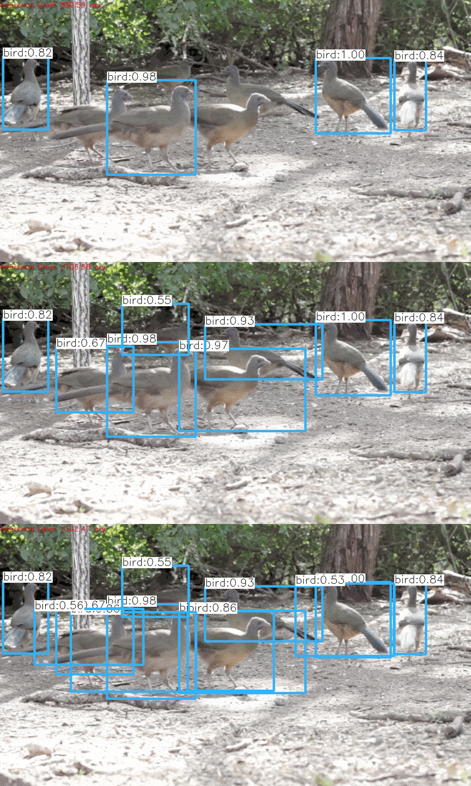
Figure 1: Effect of changing the parameter nmsThreshold
Step 4c : Draw the predicted boxes
Finally, we draw the boxes that were filtered through the non maximum suppression, on the input frame with their assigned class label and confidence scores.
Python
# Draw the predicted bounding box
def drawPred(classId, conf, left, top, right, bottom):
    # Draw a bounding box.
    cv.rectangle(frame, (left, top), (right, bottom), (255, 178, 50), 3)

    label = '%.2f' % conf

    # Get the label for the class name and its confidence
    if classes:
        assert(classId < len(classes))
        label = '%s:%s' % (classes[classId], label)

    #Display the label at the top of the bounding box
    labelSize, baseLine = cv.getTextSize(label, cv.FONT_HERSHEY_SIMPLEX, 0.5, 1)
    top = max(top, labelSize[1])
    cv.rectangle(frame, (left, top - round(1.5*labelSize[1])), (left + round(1.5*labelSize[0]), top + baseLine), (255, 255, 255), cv.FILLED)
C++
// Draw the predicted bounding box
void drawPred(int classId, float conf, int left, int top, int right, int bottom, Mat& frame)
{
    //Draw a rectangle displaying the bounding box
    rectangle(frame, Point(left, top), Point(right, bottom), Scalar(255, 178, 50), 3);

    //Get the label for the class name and its confidence
    string label = format("%.2f", conf);
    if (!classes.empty())
    {
        CV_Assert(classId < (int)classes.size());
        label = classes[classId] + ":" + label;
    }

    //Display the label at the top of the bounding box
    int baseLine;
    Size labelSize = getTextSize(label, FONT_HERSHEY_SIMPLEX, 0.5, 1, &baseLine);
    top = max(top, labelSize.height);
    rectangle(frame, Point(left, top - round(1.5*labelSize.height)), Point(left + round(1.5*labelSize.width), top + baseLine), Scalar(255, 255, 255), FILLED);
    putText(frame, label, Point(left, top), FONT_HERSHEY_SIMPLEX, 0.75, Scalar(0,0,0),1);
}
References:
We used video clips from the following sources:
Pixabay: [1], [2], [3], [4], [5], [6]
Pexels: [2]





100K+ Learners
Join Free OpenCV Bootcamp3 Hours of Learning