Deep Convolutional GAN -DCGAN – in PyTorch and TensorFlow

Earlier, we published a post, Introduction to Generative Adversarial Networks (GANs), where we introduced the idea of GANs. We also discussed its architecture, dissecting the adversarial loss function and a training strategy. We also shared code for a vanilla GAN to generate fashion images in PyTorch and TensorFlow. Now let’s learn about Deep Convolutional GAN in PyTorch and TensorFlow.

While implementing this vanilla GAN, though, we found that fully connected layers diminished the quality of generated images. 

Fully connected layers lose the inherent spatial structure present in images, while the convolutional layers learn hierarchical features by preserving spatial structures. 

Deep Convolutional Generative Adversarial Network, also known as DCGAN. This new architecture significantly improves the quality of GANs using convolutional layers. 

Some prior knowledge of convolutional neural networks, activation functions, and GANs is essential for this journey.

We will be implementing DCGAN in both PyTorch and TensorFlow, on the Anime Faces Dataset. Let’s get going!

Contents

1. Introduction
2. Types of Convolutional Layers
   1. Strided Convolutional Layer
   2. Fractionally-Strided Convolutional Layer
3. Coding DCGAN
   1. PyTorch Implementation
   2. TensorFlow Implementation

If you have not read the Introduction to GANs, you should surely go through it before proceeding with this one. 

Introduction

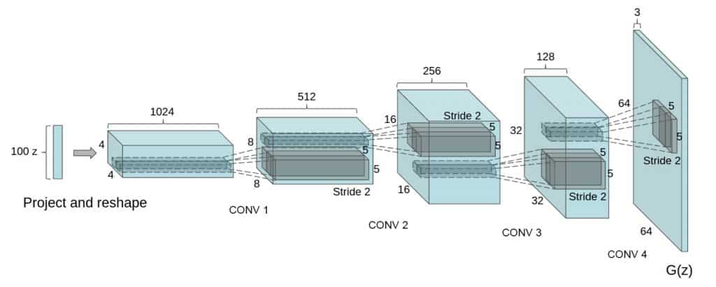
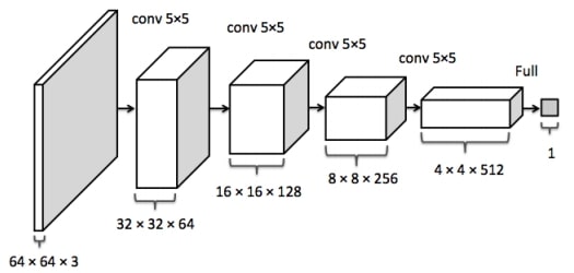
In 2016, a group of authors led by Alec Radford published a paper at the ICLR conference named Unsupervised representation learning with DCGAN.

Original GAN paper published the core idea of GAN, adversarial loss, training procedure, and preliminary experimental results.

This post is part of the series on Generative Adversarial Networks in PyTorch and TensorFlow, which consists of the following tutorials:

1. Introduction to Generative Adversarial Networks (GANs)
2. Deep Convolutional GAN in PyTorch and TensorFlow
3. Conditional GAN (cGAN) in PyTorch and TensorFlow
4. Pix2Pix: Paired Image-to-Image Translation in PyTorch & TensorFlow

DCGAN generated higher-quality images by 

1. Using strided convolutional layers in the discriminator to downsample the images.
2. Using fractionally-strided convolutional layers to upsample the images.

Let’s understand strided and fractionally strided convolutional layers then we can go over other contributions of this paper.

Types of Convolutional Layers

1. 1D, 2D, 3D Strided Convolution
2. Fractionally-Strided Convolution (Transposed Convolution)
3. Dilated Convolution (Atrous Convolution)
4. Separable Convolution (Spatially Separable Convolution)
5. Flattened Convolution
6. Grouped Convolution
7. Shuffled Grouped Convolution
8. Pointwise Grouped Convolution

Here for this post, we will pick the one that will implement the DCGAN. So, it’s only the 2D-Strided and the Fractionally-Strided Convolutional Layers that deserve your attention here.

Strided Convolutional Layer

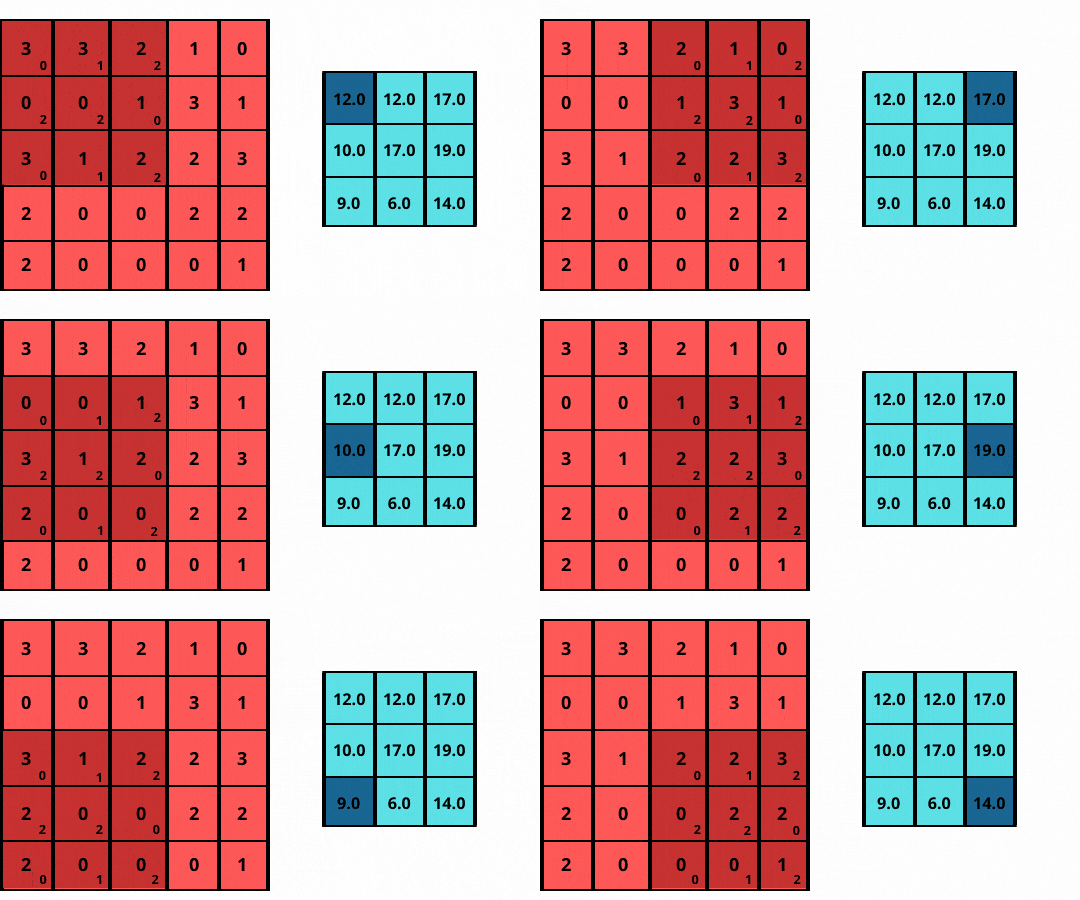
As shown in the above figure:

The images here are two-dimensional, hence, the 2D-convolution operation is applicable. The ‘convolution’ in the convolutional layer is an element-wise multiplication with a filter. It is then followed by adding up those values to get the result

• Consider a grayscale (1-channel) image sized 5 x 5 (shown on left)
• Slide a filter of size 3 x 3 (matrix) over it, having elements [[0, 1, 2], [2, 2, 0], [0, 1, 2]]. 
• The filter performs an element-wise multiplication at each position and then adds to the image.
• The final output is a 3 x 3 matrix (shown on the right). 

Note how the filter or kernel now strides with a step size of one, sliding pixel by pixel over every column for each row.

• In DCGAN, the authors used a Stride of 2, meaning the filter slides through the image, moving 2 pixels per step. 
• The authors eliminated max-pooling, which is generally used for downsampling an image. Instead, they adopted strided convolution, with a stride of 2, to downsample the image in Discriminator.

Max-pooling has no learnable parameters. Strided convolution generally allows the network to learn its own spatial downsampling.

Fractionally-Strided Convolutional Layer

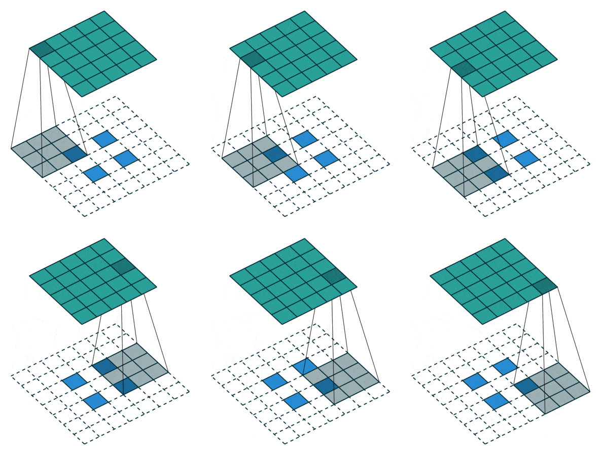
Fractionally-strided convolution, also known as transposed convolution, is the opposite of a convolution operation. 

• In a convolution operation (for example, stride = 2), a downsampled (smaller) output of the larger input is produced.
• Whereas in a fractionally-strided operation, an upsampled (larger) output is obtained from a smaller input. 

As shown in the above two figures, a 2 x 2 input matrix is upsampled to a 4 x 4 matrix. Similarly, a 2 x 2 input matrix is upsampled to a 5 x 5 matrix.

Traditional interpolation techniques like bilinear, bicubic interpolation too can do this upsampling. Why need something new then? That’s because they lack learnable parameters. In this case it cannot be trained on your data. The fractionally-strided convolution based on Deep learning operation suffers from no such issue. It easily learns to upsample or transform the input space by training itself on the given data, thereby maximizing the objective function of your overall network.

Transposed or fractionally-strided convolution is used in many Deep Learning applications like Image Inpainting, Semantic Segmentation, Image Super-Resolution etc.

In DCGAN, the authors used a series of four fractionally-strided convolutions to upsample the 100-dimensional input, into a 64 × 64 pixel image in the Generator.

For more details on fractionally-strided convolutions, consider reading the paper A guide to convolution arithmetic for deep learning.

Enough of theory, right? Let’s get our hands dirty by writing some code, and see DCGAN in action.

Coding a DCGAN in PyTorch and TensorFlow

You will code a DCGAN now, using both Pytorch and Tensorflow frameworks. So, finally, all that theory will be put to practical use. You will learn to generate anime face images, from noise vectors sampled from a normal distribution.

Dataset

Anime Face Dataset consists of 63,632 high-quality anime faces, which were scraped from getchu, then cropped using the anime face-detection algorithm. In this dataset, you’ll find RGB images:

• In various sizes, ranging from 80 – 120. Resize the images to a fixed size, only then feed into the neural network.
• Of high-quality, very colorful with white background, and having a wide range of anime characters.

Feed these images into the discriminator as real images. Once GAN is trained, your generator will produce realistic-looking anime faces, like the ones shown above.

Note: Pytorch v1.7 and Tensorflow v2.4 implementations were carried out on a 16GB Volta architecture 100 GPU, Cuda 11.0. But you can get identical results on Google Colab as well.

Click here to download the source code to this post

Pytorch Implementation

Importing Modules

# import the required packages
import torch
import argparse
import numpy as np
import torch.nn as nn
import torch.optim as optim
from torchvision import datasets, transforms
from torch.autograd import Variable
from torchvision.utils import save_image
from torchvision.utils import make_grid
from torch.utils.tensorboard import SummaryWriter

In Lines 2-11, we import the necessary packages like Torch, Torchvision, and NumPy.

Loading and Preprocessing Dataset

train_transform = transforms.Compose([transforms.Resize((64, 64)),
    transforms.ToTensor(),
    transforms.Normalize([0.5, 0.5, 0.5], [0.5, 0.5, 0.5])])
train_dataset = datasets.ImageFolder(root='anime', transform=train_transform)
train_loader = torch.utils.data.DataLoader(dataset=train_dataset, batch_size=batch_size, shuffle=True)

In Lines 12-14, you pass a list of transforms to be composed. 

• The anime face images are of varied sizes. First, resize them to a fixed size of .
• Then normalize, using the mean and standard deviation of 0.5. Note that both mean & variance have three values, as you are dealing with an RGB image.
  • The normalization maps the pixel values from the range [0, 255] to the range [-1, 1]. Mapping pixel values between [-1, 1] has proven useful while training GANs. 
• Also, convert the images to torch tensors.

Next, in Line 15, you load the Anime Face Dataset and apply the train_transform (resizing, normalization and converting images to tensors). 

Line 16 defines the training data loader, which combines the Anime dataset to provide an iterable over the dataset used while training. Here you will:

• specify the batch_size (how many images in each batch) 
• shuffle = True, which will reshuffle the data after every epoch.

Weights Initialization

# custom weights initialization called on gen and disc model
def weights_init(m):
    classname = m.__class__.__name__
    if classname.find('Conv') != -1:
        torch.nn.init.normal_(m.weight, 0.0, 0.02)
    elif classname.find('BatchNorm') != -1:
        torch.nn.init.normal_(m.weight, 1.0, 0.02)
        torch.nn.init.zeros_(m.bias)    

Define the weight initialization function, which is called on the generator and discriminator model layers. The function checks if the layer passed to it is a convolution layer or the batch-normalization layer. 

• All the convolution-layer weights are initialized from a zero-centered normal distribution, with a standard deviation of 0.02. 
• The batch-normalization layer weights are initialized with a normal distribution, having mean 1 and a standard deviation of 0.02. The bias is initialized with zeros.

Generator Network

# Generator Model Class Definition      
class Generator(nn.Module):
    def __init__(self):
        super(Generator, self).__init__()
        self.main = nn.Sequential(
            # Block 1:input is Z, going into a convolution
            nn.ConvTranspose2d(latent_dim, 64 * 8, 4, 1, 0, bias=False),
            nn.BatchNorm2d(64 * 8),
            nn.ReLU(True),
            # Block 2: input is (64 * 8) x 4 x 4
            nn.ConvTranspose2d(64 * 8, 64 * 4, 4, 2, 1, bias=False),
            nn.BatchNorm2d(64 * 4),
            nn.ReLU(True),
            # Block 3: input is (64 * 4) x 8 x 8
            nn.ConvTranspose2d(64 * 4, 64 * 2, 4, 2, 1, bias=False),
            nn.BatchNorm2d(64 * 2),
            nn.ReLU(True),
            # Block 4: input is (64 * 2) x 16 x 16
            nn.ConvTranspose2d(64 * 2, 64, 4, 2, 1, bias=False),
            nn.BatchNorm2d(64),
            nn.ReLU(True),
            # Block 5: input is (64) x 32 x 32
            nn.ConvTranspose2d(64, 3, 4, 2, 1, bias=False),
            nn.Tanh()
            # Output: output is (3) x 64 x 64
        )

    def forward(self, input):
        output = self.main(input)
        return output    

In Lines 26-50, you define the generator’s sequential model class. Note that the model has been divided into 5 blocks, and each block consists of:

• A Convolution 2D Transpose Layer
• Followed by a BatchNorm Layer and ReLU Activation Function
• And a tanh Activation Function in the last block, instead of ReLU. 

The generator is a fully-convolutional network that inputs a noise vector (latent_dim) to output an image of 3 x 64 x 64. Think of it as a decoder. Feed it a latent vector of 100 dimensions and an upsampled, high-dimensional image of size 3 x 64 x 64.

Generator Network Summary

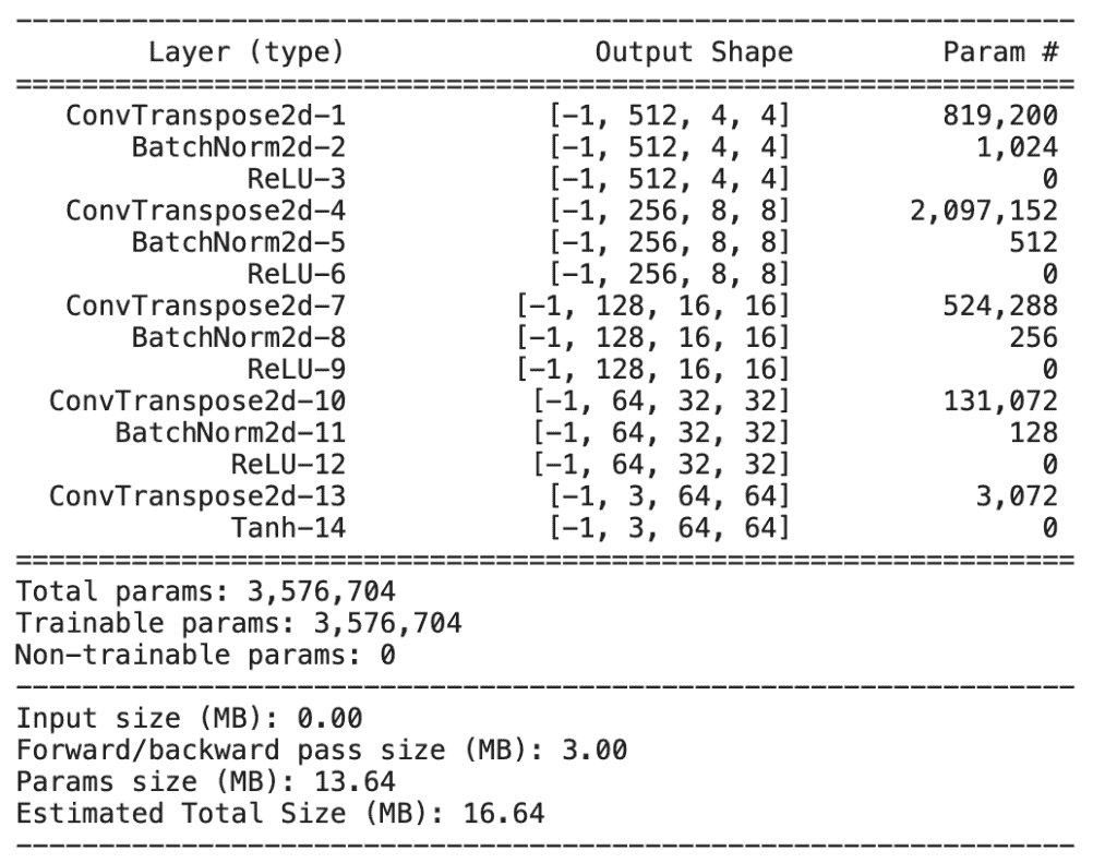
The Convolution 2D Transpose Layer has six parameters:

1. input channels
2. output channels
3. kernel or filter size
4. strides
5. padding
6. bias.

Note:

• We start with 512 output channels, and divide the output channels by a factor of 2 up until the 4th block,
• In the final block, the output channels are equal to 3 (RGB image).
• The stride of 2 is used in every layer. It doubles the input at every block, going from 4 x 4 at the first block, to 64 x 64 at the final block. 
• The tanh activation at the output layer ensures that the pixel values are mapped between .  If you recall, we normalized the images to range ) for the output of the tanh function also lies between .

The forward function of the generator, Lines 52-54 is fed the noise vector (normal distribution). This input to the model returns an image. The generator, as you know, mimics the real data distribution (anime-faces dataset), without actually seeing it.

Discriminator Network

# Discriminator Model Class Definition
class Discriminator(nn.Module):
    def __init__(self):
        super(Discriminator, self).__init__()
        self.main = nn.Sequential(
            # Block 1: input is (3) x 64 x 64
            nn.Conv2d(3, 64, 4, 2, 1, bias=False),
            nn.LeakyReLU(0.2, inplace=True),
            # Block 2: input is (64) x 32 x 32
            nn.Conv2d(64, 64 * 2, 4, 2, 1, bias=False),
            nn.BatchNorm2d(64 * 2),
            nn.LeakyReLU(0.2, inplace=True),
            # Block 3: input is (64*2) x 16 x 16
            nn.Conv2d(64 * 2, 64 * 4, 4, 2, 1, bias=False),
            nn.BatchNorm2d(64 * 4),
            nn.LeakyReLU(0.2, inplace=True),
            # Block 4: input is (64*4) x 8 x 8
            nn.Conv2d(64 * 4, 64 * 8, 4, 2, 1, bias=False),
            nn.BatchNorm2d(64 * 8),
            nn.LeakyReLU(0.2, inplace=True),
            # Block 5: input is (64*8) x 4 x 4
            nn.Conv2d(64 * 8, 1, 4, 1, 0, bias=False),
            nn.Sigmoid(),
            nn.Flatten()
            # Output: 1
        )

    def forward(self, input):
        output = self.main(input)
        return output

The discriminator is a binary classifier consisting of convolutional layers. Lines 56-79 define the sequential discriminator model, which 

• Inputs an image of dimension 3 x 64 x 64
• Outputs a score between 0 and 1
• Has Leaky-Relu (with a slope of 0.2) as an activation function in the intermediate layers
• Has a Sigmoid activation function in the output layer

Discriminator Network Summary

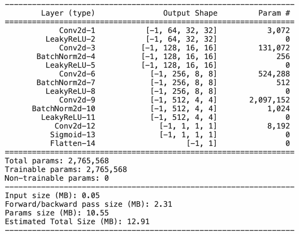
• The first block consists of a convolution layer, followed by an activation function.
• Blocks 2, 3, and 4 consist of a convolution layer, a batch-normalization layer and an activation function, LeakyReLU. 
• The last block comprises no batch-normalization layer, with a sigmoid activation function. 

You start with 64 filters in each block, then double them up till the 4th block. And finally, are left with just 1 filter in the last block.

When the forward function of the discriminator, Lines 81-83, is fed an image, it returns the output 1 (the image is real) or 0 (it is fake).

generator = Generator().to(device)
generator.apply(weights_init)
discriminator = Discriminator().to(device)
discriminator.apply(weights_init)

In Lines 84-87, the generator and discriminator models are moved to a device (CPU or GPU, depending on the hardware). The predefined weight_init function is applied to both models, which initializes all the parametric layers.

Loss Function

adversarial_loss = nn.BCELoss() 

The Binary Cross-Entropy loss is defined to model the objectives of the two networks.

Generator Loss

def generator_loss(fake_output, label):
    gen_loss = adversarial_loss(fake_output, label)
    #print(gen_loss)
    return gen_loss

The generator_loss function is fed two parameters:

• fake_output: Output predictions from the discriminator when fed generator-produced images.
• label: Ground truth labels (1), for you would like the generator to fool the discriminator and produce real images. Hence, the labels would be one.

Discriminator Loss

def discriminator_loss(output, label):
    disc_loss = adversarial_loss(output, label)
    return disc_loss

The discriminator loss has:

• the real (original images) output predictions, ground truth label as 1
• fake (generated images) output predictions, ground truth label as 0.

Twice, you’ll be calling out the discriminator loss, when training the same batch of images: once for real images and once for the fake ones.

Optimizer

learning_rate = 0.0002 
G_optimizer = optim.Adam(generator.parameters(), lr = learning_rate, betas=(0.5, 0.999))
D_optimizer = optim.Adam(discriminator.parameters(), lr = learning_rate, betas=(0.5, 0.999))

Both the generator and the discriminator are optimized with Adam optimizer. Two arguments are  passed to it:

• a learning rate of
• betas coefficients b1 (0.5) & b2 (0.999) – These compute running averages of gradients during backpropagation.

Training the Networks

Discriminator

for epoch in range(1, num_epochs+1): 
    D_loss_list, G_loss_list = [], []
   
    for index, (real_images, _) in enumerate(train_loader):
      D_optimizer.zero_grad()
      real_images = real_images.to(device)
      
      real_target = Variable(torch.ones(real_images.size(0)).to(device))
      fake_target = Variable(torch.zeros(real_images.size(0)).to(device))

      output = discriminator(real_images)
      D_real_loss = discriminator_loss(output, real_target)
      D_real_loss.backward()
 
      noise_vector = torch.randn(real_images.size(0), 100, 1, 1, device=device)  
      noise_vector = noise_vector.to(device)
      generated_image = generator(noise_vector)
      output = discriminator(generated_image.detach())
      D_fake_loss = discriminator_loss(output,fake_target)

      # train with fake
      D_fake_loss.backward()
      
      D_total_loss = D_real_loss + D_fake_loss
      D_loss_list.append(D_total_loss)
      
      D_optimizer.step()

The training procedure is similar to that for the vanilla GAN, and is done in two parts: real images and fake images (produced by the generator). 

• In each batch, you create labels: real and fake, against which loss is calculated. 
• First pass the real images through a discriminator, calculate the loss D_real_loss, and then backpropagate it through the discriminator network.

In Line 113, 

• Sample the noise vector from a normal distribution of shape batch_size x 100 x 1 x 1. 
• Pass the noise vector through the generator.
• Feed the generated image to the discriminator. 
• The D_fake_loss is then calculated and backpropagated through the discriminator network to compute the gradients.
• Finally, call the D_optimizer.step(). It updates the discriminator parameters, using the Adam optimizer.

Generator

# Train G on D's output
      G_optimizer.zero_grad()
      gen_output = discriminator(generated_image)
      G_loss = generator_loss(gen_output, real_target)
      G_loss_list.append(G_loss)

      G_loss.backward()
      G_optimizer.step()

• The feedback from the discriminator helps train the generator. 
• The images generated by the generator in Line 115 are again fed to the discriminator, which classifies them as real or fake. 

Do you remember how in the previous block, you updated the discriminator parameters based on the loss of the real and fake images? This update increased the efficiency of the discriminator, making it even better at differentiating fake images from real ones. The generator finds it harder now to fool the discriminator. And that’s what we want, right?

• The G_loss is calculated, and gradients are computed for the generator network.

Note: The generator_loss is calculated with labels as real_target ( 1 ) because you want the generator to produce real images by fooling the discriminator. 

• Finally, G_optimizer.step() optimizes the generator’s parameters.

Results

Look at the image grids below. The images in it were produced by the generator during three different stages of the training. You can see how the images are noisy to start with, but as the training progresses, more realistic-looking anime face images are generated.

TensorFlow Implementation

Let’s reproduce the PyTorch implementation of DCGAN in Tensorflow. For this, use Tensorflow v2.4.0 and Keras v2.4.3.

Importing the Packages

#import the required packages
import os
import time
import keras
import numpy as np
import tensorflow as tf
from tensorflow.keras import layers
from IPython import display
import matplotlib.pyplot as plt
%matplotlib inline

Begin by importing necessary packages like TensorFlow, TensorFlow layers, time, and matplotlib for plotting on Lines 2-10.

Data Loading and Preprocessing

train_ds = tf.keras.preprocessing.image_dataset_from_directory(
  'anime',
  image_size=(img_height, img_width),
  batch_size=batch_size,
  label_mode=None)

AUTOTUNE = tf.data.experimental.AUTOTUNE

train_ds = train_ds.cache().shuffle(1000).prefetch(buffer_size=AUTOTUNE)

normalization_layer = layers.experimental.preprocessing.Rescaling(scale= 1./127.5, offset=-1)
normalized_ds = train_ds.map(lambda x: normalization_layer(x))

• Loading the dataset is fairly simple, similar to the PyTorch data loader.
• Use the tf.keras preprocessing dataset module. It has a function image_dataset_from_directory that loads the data from the specified directory, which in our case is Anime. 
• Pass the required image_size (64 x 64 ) and batch_size (128), where you will train the model.  No labels are required to solve this problem, so the label_mode flag will be None.

We don’t want data loading and preprocessing bottlenecks while training the model simply because the data part happens on the CPU while the model is trained on the GPU hardware. So, we use buffered prefetching that yields data from disk. The I/O operations will not come in the way then. 

In Line 17:

• tf.data.experimental.AUTOTUNE prompts the tf.data runtime to tune the value dynamically at runtime. 
• The .cache() keeps the images in memory, after they are loaded off the disk, during the first epoch,
• The .prefetch() overlaps the input pipeline and model training. Consider reading TensorFlow’s official docs to understand these functions in detail.

Note: You could skip the AUTOTUNE part for it requires more CPU cores. It reserves the images in memory, which might create a bottleneck in the training. Finally, in Line 22, use the Lambda function to normalize all the input images from [0, 255] to [-1, 1], to get normalized_ds, which you will feed to the model during the training. In the Lambda function, you pass the preprocessing layer, defined at Line 21.

Generator and Discriminator Architecture

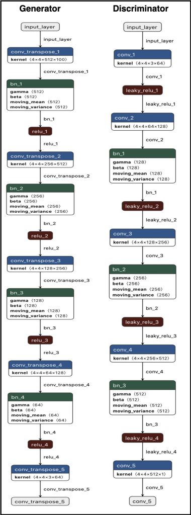
Generator Function

def generator():
    
    inputs = keras.Input(shape=(1, 1, 100), name='input_layer')
    # Block 1:input is latent(100), going into a convolution
    x = layers.Conv2DTranspose(64 * 8, kernel_size=4, strides= 4, padding='same', kernel_initializer=tf.keras.initializers.RandomNormal(
    mean=0.0, stddev=0.02), use_bias=False, name='conv_transpose_1')(inputs)
    x = layers.BatchNormalization(momentum=0.1,  epsilon=0.8, center=1.0, scale=0.02, name='bn_1')(x)
    x = layers.ReLU(name='relu_1')(x)
    
    # Block 2: input is 4 x 4 x (64 * 8)
    x = layers.Conv2DTranspose(64 * 4, kernel_size=4, strides= 2, padding='same', kernel_initializer=tf.keras.initializers.RandomNormal(
    mean=0.0, stddev=0.02), use_bias=False, name='conv_transpose_2')(x)
    x = layers.BatchNormalization(momentum=0.1,  epsilon=0.8, center=1.0, scale=0.02, name='bn_2')(x)
    x = layers.ReLU(name='relu_2')(x)
    
    # Block 3: input is 8 x 8 x (64 * 4)
    x = layers.Conv2DTranspose(64 * 2, 4, 2, padding='same', kernel_initializer=tf.keras.initializers.RandomNormal(
    mean=0.0, stddev=0.02), use_bias=False, name='conv_transpose_3')(x)
    x = layers.BatchNormalization(momentum=0.1,  epsilon=0.8,  center=1.0, scale=0.02, name='bn_3')(x)
    x = layers.ReLU(name='relu_3')(x)
  
    # Block 4: input is 16 x 16 x (64 * 2)
    x = layers.Conv2DTranspose(64 * 1, 4, 2, padding='same', kernel_initializer=tf.keras.initializers.RandomNormal(
    mean=0.0, stddev=0.02), use_bias=False, name='conv_transpose_4')(x)
    x = layers.BatchNormalization(momentum=0.1,  epsilon=0.8,  center=1.0, scale=0.02, name='bn_4')(x)
    x = layers.ReLU(name='relu_4')(x)
    
    # Block 5: input is 32 x 32 x (64 * 1)
    outputs = layers.Conv2DTranspose(3, 4, 2,padding='same', kernel_initializer=tf.keras.initializers.RandomNormal(
    mean=0.0, stddev=0.02), use_bias=False, activation='tanh', name='conv_transpose_5')(x)
    # Output: output 64 x 64 x 3
    model = tf.keras.Model(inputs, outputs, name="Generator")
    return model

The generator function is identical to the PyTorch generator class. 

A fully-convolutional network, it inputs a noise vector (latent_dim) to output an image of 64 x 64 x 3. Think of the generator as a decoder that, when fed a latent vector of 100 dimensions, outputs an upsampled high-dimensional image of size 64 x 64 x 3.

Recall, how in PyTorch, you initialized the weights of the layers with a custom weight_init() function. Similarly, in TensorFlow, the Conv2DTranspose layers are randomly initialized from a normal distribution centered at zero, with a variance of 0.02. The BatchNorm layer parameters are centered at one, with a mean of zero.

In Line 54, you define the model and pass both the input and output layers to the model. This can be done outside the function as well.

Discriminator Function

def discriminator():
    
    inputs = keras.Input(shape=(64, 64, 3), name='input_layer')
    # Block 1: input is 64 x 64 x (3)
    x = layers.Conv2D(64, kernel_size=4, strides= 2, padding='same', kernel_initializer=tf.keras.initializers.RandomNormal(
    mean=0.0, stddev=0.02), use_bias=False, name='conv_1')(inputs)
    x = layers.LeakyReLU(0.2, name='leaky_relu_1')(x)
    
    # Block 2: input is 32 x 32 x (64)
    x = layers.Conv2D(64 * 2, kernel_size=4, strides= 2, padding='same', kernel_initializer=tf.keras.initializers.RandomNormal(
    mean=0.0, stddev=0.02), use_bias=False, name='conv_2')(x)
    x = layers.BatchNormalization(momentum=0.1,  epsilon=0.8, center=1.0, scale=0.02, name='bn_1')(x)
    x = layers.LeakyReLU(0.2, name='leaky_relu_2')(x)
    
    # Block 3: input is 16 x 16 x (64*2)
    x = layers.Conv2D(64 * 4, 4, 2, padding='same', kernel_initializer=tf.keras.initializers.RandomNormal(
    mean=0.0, stddev=0.02), use_bias=False, name='conv_3')(x)
    x = layers.BatchNormalization(momentum=0.1,  epsilon=0.8, center=1.0, scale=0.02, name='bn_2')(x)
    x = layers.LeakyReLU(0.2, name='leaky_relu_3')(x)
  
    # Block 4: input is 8 x 8 x (64*4)
    x = layers.Conv2D(64 * 8, 4, 2, padding='same', kernel_initializer=tf.keras.initializers.RandomNormal(
    mean=0.0, stddev=0.02), use_bias=False, name='conv_4')(x)
    x = layers.BatchNormalization(momentum=0.1,  epsilon=0.8, center=1.0, scale=0.02, name='bn_3')(x)
    x = layers.LeakyReLU(0.2, name='leaky_relu_4')(x)
    
    # Block 5: input is 4 x 4 x (64*4)
    outputs = layers.Conv2D(1, 4, 2,padding='same', kernel_initializer=tf.keras.initializers.RandomNormal(
    mean=0.0, stddev=0.02), use_bias=False, activation='sigmoid', name='conv_5')(x)
    # Output: 1 x 1 x 1
    model = tf.keras.Model(inputs, outputs, name="Discriminator")
    return model

The discriminator is a binary classifier consisting of convolutional layers.

• The model inputs images of dimension 64 x 64 x 3, and outputs a score between 0 and 1.
• The intermediate layers have Leaky-Relu, with a slope of 0.2, as the activation function, 
• In the output layer, Sigmoid is the activation function. 
• Batchnorm layers are used in [2, 4] blocks.

Loss Function

binary_cross_entropy = tf.keras.losses.BinaryCrossentropy()

The Binary Cross-Entropy loss is defined to model the objectives of the two networks.

Generator Loss

def generator_loss(label, fake_output):
    gen_loss = binary_cross_entropy(label, fake_output)
    #print(gen_loss)
    return gen_loss

The  generator_loss function is fed fake outputs produced by the discriminator as the input to the discriminator was fake images (produced by the generator). It’s important to note that the generator_loss is calculated with labels as real_target for you want the generator to fool the discriminator and produce images, as close to the real ones as possible.

Discriminator Loss

def discriminator_loss(label, output):
    disc_loss = binary_cross_entropy(label, output)
    #print(total_loss)
    return disc_loss

Contrary to generator loss, in the discriminator_loss:

• the real (original images) output predictions are labelled as 1
• fake output predictions are labelled as 0 

The discriminator loss will be called twice while training the same batch of images: once for real images and once for the fakes.

Optimizer

learning_rate = 0.0002
generator_optimizer = tf.keras.optimizers.Adam(lr = 0.0002, beta_1 = 0.5, beta_2 = 0.999 )
discriminator_optimizer = tf.keras.optimizers.Adam(lr = 0.0002, beta_1 = 0.5, beta_2 = 0.999 )

The generator and discriminator are optimized with the Adam optimizer. Two arguments are passed to the optimizer: 

• a learning rate of ,
• betas coefficients b1 ( 0.5 ) & b2 ( 0.999 ) – These compute the running averages of the gradients during backpropagation.

Training the Discriminator and Generator Network in Tandem

# Notice the use of `tf.function`
# This annotation causes the function to be "compiled".
@tf.function
def train_step(images):
    # noise vector sampled from normal distribution
    noise = tf.random.normal([BATCH_SIZE, 1, 1, latent_dim])

    # Train Discriminator with real labels
    with tf.GradientTape() as disc_tape1:
        generated_images = generator(noise, training=True)

        
        real_output = discriminator(images, training=True)
        real_targets = tf.ones_like(real_output)
        disc_loss1 = discriminator_loss(real_targets, real_output)
        
    # gradient calculation for discriminator for real labels    
    gradients_of_disc1 = disc_tape1.gradient(disc_loss1, discriminator.trainable_variables)
    
    # parameters optimization for discriminator for real labels   
    discriminator_optimizer.apply_gradients(zip(gradients_of_disc1,\
    discriminator.trainable_variables))
    
    # Train Discriminator with fake labels
    with tf.GradientTape() as disc_tape2:
        fake_output = discriminator(generated_images, training=True)
        fake_targets = tf.zeros_like(fake_output)
        disc_loss2 = discriminator_loss(fake_targets, fake_output)
    # gradient calculation for discriminator for fake labels 
    gradients_of_disc2 = disc_tape2.gradient(disc_loss2, discriminator.trainable_variables)
    
    
    # parameters optimization for discriminator for fake labels        
    discriminator_optimizer.apply_gradients(zip(gradients_of_disc2,\
    discriminator.trainable_variables))
    
    # Train Generator with real labels
    with tf.GradientTape() as gen_tape:
        generated_images = generator(noise, training=True)
        fake_output = discriminator(generated_images, training=True)
        real_targets = tf.ones_like(fake_output)
        gen_loss = generator_loss(real_targets, fake_output)

    # gradient calculation for generator for real labels     
    gradients_of_gen = gen_tape.gradient(gen_loss, generator.trainable_variables)
    
    # parameters optimization for generator for real labels
    generator_optimizer.apply_gradients(zip(gradients_of_gen,\
    generator.trainable_variables))    

Do not get intimidated by the above code. Read the comments attached to each line, relate it to the GAN algorithm, and wow, it gets so simple!

The train_step function is the core of the whole DCGAN training; this is where you combine all the functions you defined above to train the GAN. 

Note the use of @tf.function in Line 102.

• This compiles the train_step function into a callable TensorFlow graph
• Also, speeds up the training time (check it out yourself).

The training of DCGAN in TensorFlow can be divided into three phases: 

• Update discriminator parameters with labels marked real
• Update discriminator parameters with fake labels
• Finally, update generator parameters with labels that are real

In the training loop: 

• First, sample the noise from a normal distribution and feed it to the generator as input. 
• The generator the model then produces an image. 
• The discriminator model is
  • First, fed real images (Line 112), based on which loss is computed with real labels, and its parameters are optimized. 
  • Then fed images (Line 125) were produced by the generator model. Fake labels helped in loss computation and parameter optimization.
• Finally, for training the generator, the generator model produces images (Line 138) for the second time. Feed these to the discriminator. Compute loss with real labels, and the parameters optimized.

Calculate the loss for each of these models: gen_loss and disc_loss. Compute the gradients, and use the Adam optimizer to update the generator and discriminator parameters.

def train(dataset, epochs):
  for epoch in range(epochs):
    start = time.time()
    for image_batch in dataset:
      train_step(image_batch)

    print ('Time for epoch {} is {} sec'.format(epoch + 1, time.time()-start))


train(normalized_ds, 100)

Finally, it’s time to train our DCGAN model in TensorFlow. The above train function takes the normalized_ds and Epochs (100) as the parameters and calls the function at every new batch, in total ( Total Training Images / Batch Size). The training is fast, and each epoch took around 24 seconds to train on a Volta 100 GPU.

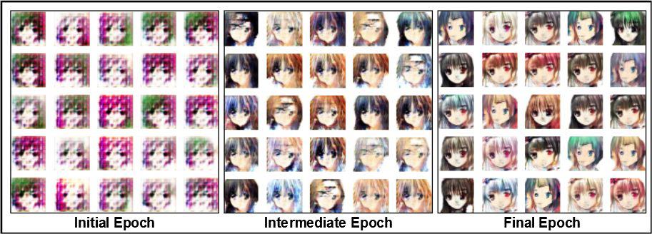
Results

Check out the image grids below. Generators at three different stages of training produced these images. As in the PyTorch implementation, here, too you find that initially, the generator produces noisy images, which are sampled from a normal distribution. As the training progresses, you get more realistic anime face images.

Conclusion

It’s a feat to have made it till here! You’ve covered a lot, so here’s a quick summary:

1. Introduction to DCGAN.  Saw how different it is from the vanilla GAN. You also understood why it generates better and more realistic images.
2. Learned about experimental studies by the authors of DCGAN, which are fairly new in the GAN regime.
3. We Discussed convolutional layers like Conv2D and Conv2D Transpose, which helped DCGAN succeed.
4. Then we implemented DCGAN in PyTorch, with Anime Faces Dataset.
5. Finally, you also implemented DCGAN in TensorFlow, with Anime Faces Dataset, and achieved results comparable to the PyTorch implementation.

You have come far. Hope it helps you stride ahead towards bigger goals.

Other Contributions of the DCGAN paper

Good papers not only give you new ideas, but they also give you details about the author’s thought process, how they went about verifying their hunches, and what experiments they did to see if their ideas were sound.  

The DCGAN paper contains many such experiments. 

After completing the DCGAN training, the discriminator was used as a feature extractor to classify CIFAR-10, SVHN digits dataset. This was the first time DCGAN was trained on these datasets, so the authors made an extra effort to demonstrate the robustness of the learned features.

After visualizing the filters learned by the generator and discriminator, they showed empirically how specific filters could learn to draw particular objects.

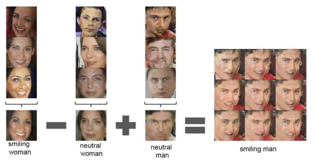
They found that the generators have interesting vector arithmetic properties, which could be used to manipulate several semantic qualities of the generated samples. Below is an example that outputs images of a smiling man by leveraging the vectors of a smiling woman. Subtracting from vectors of a neutral woman and adding to that of a neutral man gave us this smiling man.

Finally, they showed their deep convolutional adversarial pair learned a hierarchy of representations, from object parts (local features) to scenes (global features), in both the generator and the discriminator. 

We recommend you read the original paper, and we hope going through this post will help you understand the paper. 

References

• Unsupervised Representation Learning with Deep Convolutional Generative Adversarial Networks
• A Comprehensive Introduction to Different Types of Convolutions in Deep Learning
• GitHub: conv_arithmetic
• Better performance with the tf.data API