In the previous post, we learned how to classify arbitrarily sized images and visualized the response map of the network.

In Figure 1, notice that the head of the camel is almost not highlighted, and the response map contains a lot of the sand texture instead. The bounding box is also significantly off.
Something is not right.
The ResNet18 network we used is very accurate, and in fact it classifies the image correctly. Looking at the bounding box you may be tempted to think that we just got lucky and the classification was correct even when the network did not choose the best information from the image.
But is it really so? The short answer is NO. In the previous post, we used a quick and dirty approach to find the area of interest.
In this post, we will do it the right way and understand the concept of receptive fields in a neural network along the way.
Neural Network Receptive Field
Recall how we found the area of interest and bounding box around the camel in the previous post. We upsampled the response map for the predicted class to fit the original image.
That approach provided some insight, but it was strictly not the right way.
To understand how to do it the right way, we need to understand a concept called the receptive field. For a pixel in a feature map inside the network, the receptive field represents all the pixels from the previous feature maps that affected its value.
The receptive field is the proper tool to understand what the network “saw” and analyzed to predict the “camel” class, whereas the scaled response map we saw in the previous post is only a rough approximation of it.
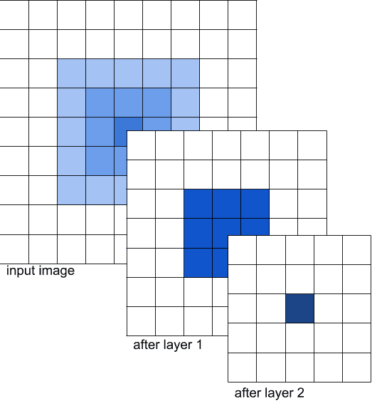
Let’s pick a toy example.
In Figure 2, we are showing the input image followed by the outputs of two layers of a Convolutional Neural Network (CNN). Let’s call the output after the first layer FEATURE_MAP_1, and the output after the second layer FEATURE_MAP_2.
Let’s suppose that the layers 1 and 2 are convolutional with kernel size 3. So, the feature map after a particular layer is affected by a 3×3 region ( i.e. 9 values ) in the previous feature map.
We want to find the receptive field of the dark blue pixel of FEATURE_MAP_2.
The value of this pixel is affected by the 9 corresponding values from the FEATURE_MAP_1 marked in blue. In turn, these 9 values are affected by the corresponding pixels from the input image.
In other words, a pixel in FEATURE_MAP_2 is affected by a 5×5 patch (marked in light blue) in the input image. These are the pixels that the dark blue one can “see” on the input image.
Note that in the input image, pixels have different shades of blue. These shades represent the number of time the corresponding pixels participated in the convolutions that affected the dark blue pixel of interest. The outer pixels were used in the computations only once. The center pixel participated in every convolution and we did 9 of them to compute FEATURE_MAP_1.
This toy example gives us an idea on how to compute the receptive field of a more complex network. By doing this, we can understand which pixels of the input image could affect the results of the network! And thus we can have a much deeper understanding of the results of the network.
Knowing the receptive field size is very useful for neural network debugging as it gives you an insight into how the net makes its decisions.
What does the Receptive Field Size Depend on?
The receptive field size of the output pixels is typically pretty large – it’s typically hundreds of pixels wide. This value depends on the depth of the network, the size of the convolutions in it, the stride, and padding used in the convolution filters. The deeper the network, the more context every pixel can “see” on the input image.
Importantly, the receptive field does not depend on the size of the input image. Even though fully convolutional nets can accept and process images of any size, their receptive field stays the same – as their depth remains constant. Sometimes this means that nets can perform badly if the objects in the input image are too large – they just won’t see enough context to make the decision!
The receptive field size also does not depend on the values of the weights in the network. In fact, it would be the same for trained and untrained networks of the same architecture.
We’ll use this fact to compute the size of the receptive field.
Receptive Field Computation for Max Activated Pixel
Let’s discuss how we can visualize the receptive field of a pixel.
There are two main ways
- Run a backpropagation for this pixel.
- Compute the receptive field size analytically.
In this post, we’ll discuss the first way, and will cover the latter in a future post.
Let’s again infer the network on our image and get the final activation map (we’ll call it “score map” here).
# Load modified resnet18 model with pretrained ImageNet weights
model = FullyConvolutionalResnet18(pretrained=True).eval()

# Perform the inference.
# Instead of a 1x1000 vector, we will get a
# 1x1000xnxm output ( i.e. a probability map
# of size n x m for each 1000 class,
# where n and m depend on the size of the image.)
preds = model(image)
preds = torch.softmax(preds, dim=1)

# Find the class with the maximum score in the n x m output map
pred, class_idx = torch.max(preds, dim=1)

row_max, row_idx = torch.max(pred, dim=1)
col_max, col_idx = torch.max(row_max, dim=1)
predicted_class = class_idx[0, row_idx[0, col_idx], col_idx]

# Find the n x m score map for the predicted class
score_map = preds[0, predicted_class, :, :].cpu()
print('Score Map shape : ', score_map.shape)
Our score map has 1 channel because we already extracted only the channel corresponding to the predicted class out of 1000 initial channels. It has 3 rows and 8 columns.
Now let’s first find the pixel in the network result with the highest value for the “camel” class. This is the pixel that got activated the most – let’s see, what parts of the image could it “see”.
scoremap_max_row_values, max_row_id = torch.max(scoremap, dim=1)
_, max_col_id = torch.max(scoremap_max_row_values, dim=1)
max_row_id = max_row_id[0, max_col_id]

print('Coords of the max activation:', max_row_id.item(), max_col_id.item())
In our image, the pixel with the highest activation is located in the 1st row and the 6th column.
Use Backprop to Compute the Receptive Field
To compute the receptive field size using backpropagation, we’ll exploit the fact that the values of the weights of the network are not relevant for computing the receptive field.
Let’s go over the steps
1. Load Model
First we load the model and put in in train mode. This ensures we will be able to pass the gradients.
# Initialize the model
model = FullyConvolutionalResnet18()
# model should be in the train mode to be able to pass the gradient
model = model.train()
2. Set Layer Parameters
As mentioned earlier, the receptive field does not depend on the weights and biases. We will exploit this fact to compute the receptive field.
As we know, convolutional layers have two parameters — weight and bias. We’ll change the weight every layer to be 0.05 and the bias to be 0.
The BatchNorm layer has four parameters — weight, bias, running_mean, and running_var. We set the weight to 0.05, bias to 0, running_mean to 0, and running_var to 1.
Here’s the code.
for module in model.modules():
    # skip errors on container modules, like nn.Sequential
    try:
        # Make all convolution weights equal.
        # Set all biases to zero.
        nn.init.constant_(module.weight, 0.05)
        nn.init.zeros_(module.bias)

        # Set BatchNorm means to zeros,
        # variances - to 1.
        nn.init.zeros_(module.running_mean)
        nn.init.ones_(module.running_var)
    except:
        pass
3. Freeze BatchNorm Layers
In the BatchNorm layer, two out of these four parameters are learnable (weight and bias), and the other two are statistics that are calculated during the forward pass. So they change the value of the input tensor, but they are not updated with the backpropagation. So even though we’ve initialized these parameters in the code above, they will be updated during the forward pass and this will adversely affect the visualization we want.
So, we should switch them to the eval mode. This way, the parameters will not be updated during a forward pass.
    # Freeze the BatchNorm stats.
    if isinstance(module, torch.nn.modules.BatchNorm2d):
        module.eval()
4. Input a white image
We want to create a situation in which the gradient at the output of the model depends only on the location of the pixels. So, we pass a white image into the network.
input = torch.ones_like(image, requires_grad=True)
out = model(input)
An important thing here is that we want to propagate the gradient to the image to see which pixels affected the final result. So, unlike the ordinary training, we’ve marked the image as differentiable for the PyTorch Autograd using by setting requires_grad to True. This way it won’t only compute the gradients for the weights of the network, but also for the image itself.
5. Tweak output gradients and backpropagate
Next we will tweak the output gradient that will be backpropagated through the network. We only want to compute the receptive field of the most activated pixel – so we’ll set the corresponding gradient value to 1 and all the others to 0.
When we backpropagate this gradient all the way to the input layer, the receptive field will light up and everything else will be dark.
Now let’s infer this synthetic image through our synthetic network.
# Set the gradient to 0.
# Only set the pixel of interest to 1.
grad = torch.zeros_like(out, requires_grad=True)
grad[0, 0, max_row_id, max_col_id] = 1

# Run the backprop.
out.backward(gradient=grad)

# Retrieve the gradient of the input image.
gradient_of_input = input.grad[0, 0].data.numpy()
# Normalize the gradient.
gradient_of_input = gradient_of_input / np.amax(gradient_of_input)
6. Visualize Results
The final step is to simply normalize the backpropagated gradient at the input layer. The normalization simply involves subtracting the minimum value and then dividing by the maximum value so the normalized image is between 0 and 1.
This normalized image is used as a mask and multiplied with the original image.
def normalize(activations):
    # transform activations so that all the values be in range [0, 1]
    activations = activations - np.min(activations[:])
    activations = activations / np.max(activations[:])
    return activations


def visualize_activations(image, activations):
    activations = normalize(activations)

    # replicate the activations to go from 1 channel to 3
    # as we have colorful input image
    # we could use cvtColor with GRAY2BGR flag here, but it is not
    # safe - our values are floats, but cvtColor expects 8-bit or
    # 16-bit inttegers
    activations = np.stack([activations, activations, activations], axis=2)
    masked_image = (image * activations).astype(np.uint8)

    return masked image


receptive_field_mask = visualize_activations(image, gradient_of_input)
cv2.imshow("receiptive_field_max_activation", receptive_field_mask)
cv2.waitKey(0)
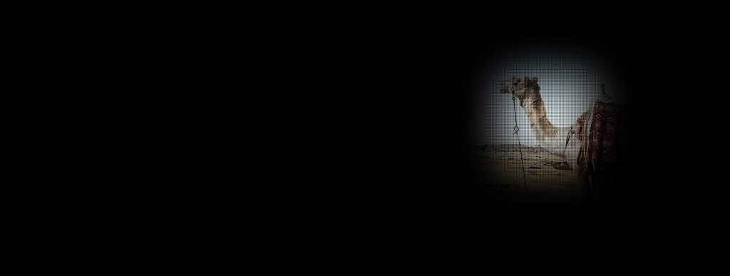
The receptive field clearly shows that the network does pays the most attention to the head of the camel! That’s good news – this means the network is smarter than we saw before.
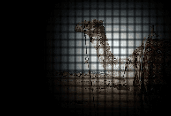
What do we see the grids?
A peculiar detail of this receptive field is its grid structure. This structure is explained by the architecture of the first layers of the ResNet. The first block runs a 7×7 convolution on the input data and then quickly downsamples it to decrease the computations. This means that we only look once at the high-quality image and then look many more times to progressively downsampled one. In terms of the receptive field, this means that the regions that only participate in the first convolution and then get cut by the downsampling operation only affect the result in a subtle way – and thus are represented as the dark grid lines here.
Receptive Field for the Net Prediction
Let’s go further and analyze not the most activated pixel, but the whole network feature map for the class “camel”. In fact, we can backpropagate it the same way we did for a single pixel – we just need to put the whole tensor to the output gradient. This way we’ll understand which pixels from the input image resulted in the whole final score map for the camel class.
out = model(input)
grad = torch.zeros_like(out, requires_grad=True)
grad[0, predicted_class] = scoremap

out.backward(gradient=grad)
gradient_of_input = input.grad[0, 0].data.numpy()
gradient_of_input = gradient_of_input / np.amax(gradient_of_input)
The resulting image shows which areas of the input image affected the prediction of the network:
def find_rect(activations):
    # Dilate and erode the activations to remove grid-like artifacts
    kernel = np.ones((5, 5), np.uint8)
    activations = cv2.dilate(activations, kernel=kernel)
    activations = cv2.erode(activations, kernel=kernel)

    # Binarize the activations
    _, activations = cv2.threshold(activations, 0.25, 1, type=cv2.THRESH_BINARY)
    activations = activations.astype(np.uint8).copy()

    # Find the countour of the binary blob
    contours, _ = cv2.findContours(activations, mode=cv2.RETR_EXTERNAL, method=cv2.CHAIN_APPROX_SIMPLE)

    # Find bounding box around the object.
    rect = cv2.boundingRect(contours[0])

    return Rect(rect[0], rect[1], rect[0] + rect[2], rect[1] + rect[3])

rect = find_rect(gradient_of_input)
receptive_field_mask = visualize_activations(image, gradient_of_input)

cv2.rectangle(receptive_field_mask, (rect.x1, rect.y1), (rect.x2, rect.y2), color=(0, 0, 255), thickness=2)

cv2.imshow("receiptive_field", receptive_field_mask)
cv2.waitKey(0)
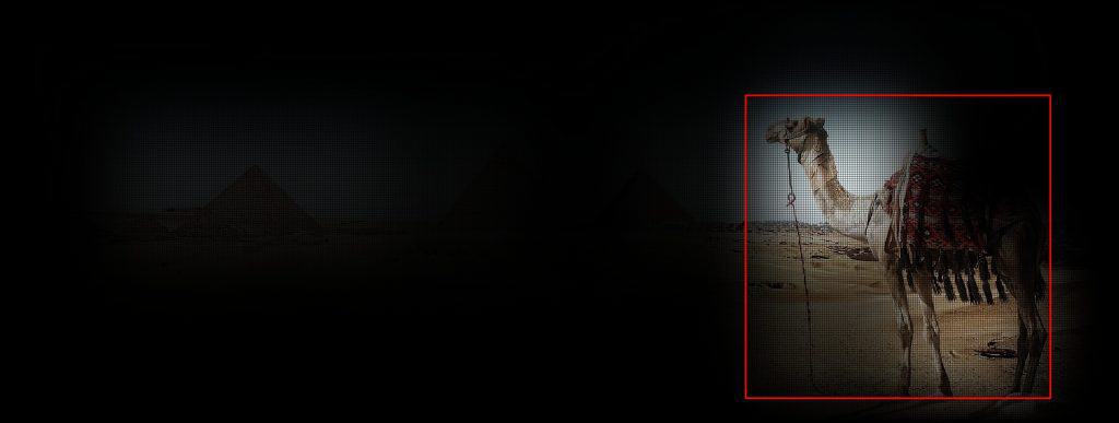
Please note that having nonzero values somewhere in this feature map does not mean that the network predicts camel class for that position – activations for the other classes may be much higher.
Let’s also compare this image to the scaled score map that we used as a rough approximation of the receptive field before:

Now we see good news here. First, the bounding box here is tighter wrt the camel – so our network is actually even better an object detector than we thought before. Second, the areas that affected the correct prediction seem even more relevant in the receptive field visualization than in the approximated score map one.









100K+ Learners
Join Free OpenCV Bootcamp3 Hours of Learning