


In our recent post about receptive field computation, we examined the concept of receptive fields using PyTorch.
We learned receptive field is the proper tool to understand what the network ‘sees’ and analyze to predict the answer, whereas the scaled response map is only a rough approximation of it.
Several readers of the PyTorch post requested a similar post using Tensorflow / Keras. So by popular demand, we are going to solve the same problem using TensorFlow, paying attention to the TF task implementation part.
In this post we are going to solve the same problem using TensorFlow, paying attention to the TF task implementation part.
TensorFlow FCN Receptive Field
In the early post we found out that the receptive field is a useful way for neural network debugging as we can take a look at how the network makes its decisions. Let’s implement the visualization of the pixel receptive field by running a backpropagation for this pixel using TensorFlow.
The first step we need to do is to get the inference of the previously discussed TensorFlow FCN ResNet-50 on the camel image as we need to obtain the prediction score map:

    # read ImageNet class ids to a list of labels
    with open("imagenet_classes.txt") as f:
        labels = [line.strip() for line in f.readlines()]

    # convert image to the RGB format
    image = cv2.cvtColor(original_image, cv2.COLOR_BGR2RGB)

    # TF pre-process image
    image = preprocess_input(image)

    # convert image to NCHW tf.tensor
    image = tf.expand_dims(image, 0)

    # load resnet50 model with pretrained ImageNet weights
    model = fully_convolutional_resnet50(
        input_shape=(image.shape[-3:])
    )

    # Perform inference.
    # Instead of a 1×1000 vector, we will get a
    # 1×1000×n×m output ( i.e. a probability map
    # of size n × m for each 1000 class,
    # where n and m depend on the size of the image).
    preds = model.predict(image)
    preds = tf.transpose(preds, perm=[0, 3, 1, 2])
    preds = tf.nn.softmax(preds, axis=1)
    print("Response map shape : ", preds.shape)

    # find class with the maximum score in the n × m output map
    pred = tf.math.reduce_max(preds, axis=1)
    class_idx = tf.math.argmax(preds, axis=1)

    row_max = tf.math.reduce_max(pred, axis=1)
    row_idx = tf.math.argmax(pred, axis=1)

    col_idx = tf.math.argmax(row_max, axis=1)

    predicted_class = tf.gather_nd(
        class_idx,
        (0, tf.gather_nd(row_idx, (0, col_idx[0])), col_idx[0]),
    )

    # print the top predicted class
    print("Predicted Class : ",
        labels[predicted_class], predicted_class)

    # find the n × m score map for the predicted class
    score_map = tf.expand_dims(
        preds[0, predicted_class, :, :], 0).numpy()
    print("Score Map shape : ", score_map.shape)
The output is:
Response map shape :  (1, 1000, 3, 8)
Predicted Class :  Arabian camel, dromedary, Camelus dromedarius tf.Tensor(354, shape=(), dtype=int64)
Score Map shape :  (1, 3, 8)
The score map has 1 channel, which was extracted due to its accordance with the predicted class out of 1000 initial classes.
The below code finds the most activated pixel in the network – the pixel with the highest activation value for the ‘camel’ class:
scoremap_max_row_values = tf.math.reduce_max(scoremap, axis=1)
max_row_id = tf.math.argmax(scoremap, axis=1)
max_col_id = tf.math.argmax(scoremap_max_row_values,
    axis=1).numpy()[0]
max_row_id = max_row_id[0, max_col_id].numpy()
print(
    "Coords of the max activation:", max_row_id, max_col_id,
)
The result is the 1-st row and the 6-th column:
Coords of the max activation: 1 6Compute The Receptive Field Computation with Backprop
The first step to compute the backpropagation receptive field is to load the model. We use an untrained model for the further subtle configuration of the layers:
def backprop_receptive_field(
    image, predicted_class, scoremap, use_max_activation=False,
):
    model = fully_convolutional_resnet50(
        input_shape=(image.shape[-3:]),
        pretrained_resnet=False,
    )
It should be noticed that the receptive field does not depend on the weights and biases. Thus, we will change the configuration of convolutional and batch normalization layers, so they all have the same values:
- convolutional layers denoted by
Conv2D: set the weights to 0.005 and the bias to 0 BatchNormalizationlayers: set weight, bias, running mean, and running variance parameters to 0.05, 0, 0, 1 accordingly.


for module in model.layers:
    try:
        if isinstance(module, Conv2D):
            conv_weights = np.full(module.get_weights()[0].shape,
                0.005)
            if len(module.get_weights()) > 1:
                conv_biases = np.full(module.get_weights()[1].shape,
                    0.0)
                module.set_weights([conv_weights, conv_biases])
            # cases when use_bias = False
            else:
                module.set_weights([conv_weights])
        if isinstance(module, BatchNormalization):
            # weight sequence: gamma, beta, running mean, running variance
            bn_weights = [
                module.get_weights()[0],
                module.get_weights()[1],
                np.full(module.get_weights()[2].shape, 0.0),
                np.full(module.get_weights()[3].shape, 1.0),
            ]
            module.set_weights(bn_weights)
    except:
        pass
Create an empty white image to pass into the network as gradients need to be dependent only on the location of the pixels:
input = tf.ones_like(image)
out = model.predict(image)
To get the receptive field of the most activated pixel we need to set the corresponding gradient value to 1 and all the others to 0. These appropriate values are denoted by receptive_field_mask (see the code below). Let’s view the inference step with the empty synthetic image as input:
receptive_field_mask = tf.Variable(tf.zeros_like(out))

if not use_max_activation:
    receptive_field_mask[:, :, :, predicted_class].
        assign(scoremap)
else:
    scoremap_max_row_values = tf.math.reduce_max(
        scoremap,
        axis=1
    )
    max_row_id = tf.math.argmax(scoremap, axis=1)
    max_col_id = tf.math.argmax(scoremap_max_row_values,
        axis=1).numpy()[0]
    max_row_id = max_row_id[0, max_col_id].numpy()
    print(
        "Coords of the max activation:", max_row_id, max_col_id,
    )
    # update grad
    receptive_field_mask = tf.tensor_scatter_nd_update(
        receptive_field_mask,
        [(0, max_row_id, max_col_id, 0)], [1],
    )
The gradients computation phase:
grads = []
with tf.GradientTape() as tf_gradient_tape:
    tf_gradient_tape.watch(input)
    # get the predictions
    preds = model(input)
    # apply the mask
    pseudo_loss = preds * receptive_field_mask
    pseudo_loss = K.mean(pseudo_loss)
    # get gradient
    grad = tf_gradient_tape.gradient(pseudo_loss, input)
    grad = tf.transpose(grad, perm=[0, 3, 1, 2])
    grads.append(grad)
return grads[0][0, 0]
For tracing a tensor by tf_gradient_tape we should invoke the watch() function. In our case we needed to trace our input, which is the empty image defined before the tf.GradientTape() call.
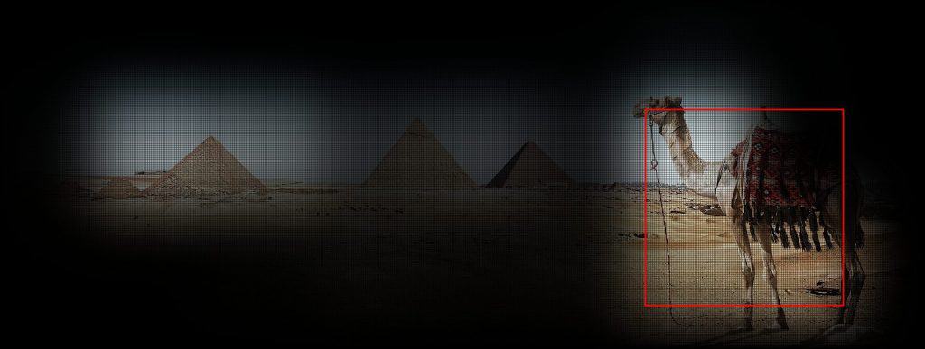
Let’s visualize the result – the receptive field for the most activated pixels, which are located around the camel’s head:

To analyze the whole network feature map for the ‘camel’ class, we need to put the whole tensor to the output gradient:
if not use_max_activation:
    receptive_field_mask[:, :, :, predicted_class].
        assign(scoremap)
The result is:
By looking at it, we can understand which pixels from the input image resulted in the final score map for the dromedary class.
As we can observe from the outputs, the bounding box in the last experiment is tighter, hence initially the model works better than we could conclude after the experiments in TF FCN ResNet50 article:
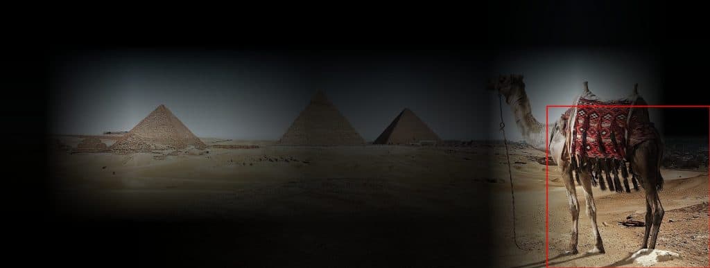
Also the regions, which depict correct predictions are more accurate in the receptive field visualization than in the approximated score map.