You can scarcely find a good article on deploying computer vision systems in industrial scenarios. So, we decided to write a blog post series on the topic.
The topics we will cover in this series are:
Part 1: Building industrial embedded deep learning inference pipelines with TensorRT in python
Part 2: Building industrial embedded deep learning inference pipelines with TensorRT in C++
Part 3: Building industrial computer vision pipelines with Vision Programming Interface (VPI)
Part 4: Using real-time Linux kernel on embedded devices for safety-critical applications.
This post will first explain how building industrial-grade computer vision products differ from creating a tech demo. Then we dive deep into TensorRT, NVIDIA’s software framework for edge AI acceleration, designed to be used in the industry.
As a gentle introduction, we will use TensorRT’s python API to demonstrate the concepts behind TensorRT and how they tie together to create an industrial application.
- How is industrial embedded computer vision different?
- Introduction to NVIDIA Jetson AGX Xavier
- What does TensorRT do?
- Introduction to TensorRT API concepts
- Semantic segmentation
- Creating inference pipeline
- Results
- Summary
1. How is industrial embedded computer vision different?
Regular readers of the LearnOpenCV blog and students taking our courses are probably well on their way to acquiring ‘hot’ computer vision and machine learning skills required in many industries today.
Suppose a company hires you, and you come up with a brilliant computer vision-based solution to some long-standing problem. For illustration, let’s assume you are automating part identification inside a factory using object detection. Your boss or customers may have no idea about what is possible with computer vision, and they may be initially skeptical. Your boss will first ask you to develop a ‘Proof of Concept’ or POC to show that your idea works.
Typically, customers (or the sales guys in your own company) require a POC before they agree to invest their time and money in buying/testing new ideas. You will be asked just to prove some critical functionality rather than create a finished product at this stage. If your demo is successful and your customers agree to buy a product based on it, you will get a chance to develop a product. The purpose of this section is to introduce you to the differences between a POC and a product.

As the name suggests, a POC is a working demo of an idea that you will quickly put together using open source/readily available software and hardware components. Even if you need to write custom code for the POC, you will maximize developer productivity above speed by writing code in python as much as possible. It doesn’t matter if the demo fails when a camera is not connected.
“Of course, the damn thing fails when there is no camera! What else do you expect?”
A POC is not a perfect product. It is just proof that an idea works.
On the other hand, a product is a different ball game entirely. Here are five differences between a POC and a product:
- Safety: An industrial product must conform to stringent safety standards. For example, If your application fails with no camera, it must fail gracefully without crashing the whole system. There are well-established safety standards such as ISO 26262 and ASIL (Automotive Safety Integrity Level) for industries like autonomous driving. When converting your POC into a product, your software will have to conform to a safety standard relevant to your industry.
- Evaluation: A POC answers only one fundamental question: Does the idea work? On the other hand, a product is evaluated on many criteria, such as latency, throughput (frames per second), reliability, and cost, to name a few. Thus, code efficiency and determinism in code execution become essential.
- Functionality: In our example of detecting parts in a factory, you might fine-tune an object detector from Tensorflow Hub or an open-source repo on GitHub with a few hundred labeled examples and show that the architecture can successfully detect objects on validation data. Demonstrating your ‘core’ idea is usually enough for a POC. However, for a product, you will have to develop the entire image-processing pipeline from frame capture to lens distortion correction to rectification and communicating the results. While it might seem that these are just one line calls to OpenCV functions, this is far from the truth. Just grabbing a frame from an industrial camera and getting it into a cv::Mat format can require several hundreds of lines of code using low-level SDKs for industrial cameras provided by respective manufacturers (common examples are Basler’s pylon and FLIR’s Spinnaker SDKs).
- Development language: As mentioned earlier, you maximize developer productivity for a POC and are encouraged to use a high-level language such as Python. However, stringent safety standards may require you to use another language such as C++ or even C for product development. For example, the autonomous driving industry develops its software almost entirely in C++ (sometimes in MISRA C) and not Python since Python is not compliant with the ISO 26262 standard. Besides mandatory standards, your company will likely have its internal programming guidelines for ensuring bug-free code.
- Licensing: So, you used an open-source object detector to prove your idea, and now you want to use it in a product. You don’t want your competitors to know all your secrets, so you want to keep the source code of your product closed. With few exceptions, licensing isn’t a problem to be thought of deeply for POC. Still, when you decide to make a commercial product based on open source components, you must ensure you don’t violate any original license terms. For example, suppose you used code released under the GNU Public License (GPL) in your project. In that case, you are legally bound to open source the entirety of your project under the same license (implying that you can’t use GPL code in a closed source setting). Differing restrictions on commercial use, patenting, etc., exist for most open source licenses. Even if some functionality is available open-source, you might still be required to implement it from scratch, so you are not bound by the original terms.
2. Introduction to NVIDIA Jetson AGX Xavier
NVIDIA is the leading vendor of hardware accelerators for AI training and inference. In the rest of this blog post, we will build upon the ideas of production quality machine learning introduced in the previous section and show you how to create production-ready deep learning applications. Deployment is a vast topic, and we cannot fully cover it in just one blog post, so to keep things manageable, we will proceed in steps. The purpose of today’s post is to introduce NVIDIA’s TensorRT (TRT) framework for accelerating deep learning inference. The industry has widely adopted TRT, and familiarity with TRT is essential for a computer vision engineer looking to deploy complex models into production.
For this blog post, we will use an embedded board, specifically NVIDIA Jetson AGX Xavier (JAX), but the concepts of TRT we will learn also apply equally to datacenter applications. You can use the contents you learn in this blog post to accelerate inference on a cloud application utilizing a datacenter GPU that gets raw data from multiple edge devices and performs inference in a centralized fashion to provide real-time insights.
An example of such an application could be a central traffic monitoring system in a smart city that needs to monitor traffic in real-time to create a traffic density map and identify bottlenecks.
Everything we will cover will also work on other Jetson boards like Jetson Xavier NX. With two exceptions (int8 precision and DLA inference), you will be able to run all the code on the much more affordable Jetson Nano as well. We purposefully deviate from the most affordable Jetson board because the nano board is just a learning tool, and we never use it in an industrial product. Finally, people interested in automotive applications like autonomous driving will be thrilled to know that the code in this post will also work on the NVIDIA Drive PX.
The AGX SoC (system on chip) is a full-fledged solution for creating industrial edge AI products. It has a 512-core Volta generation GPU and an 8-core Carmel CPU. Most introductions to Jetson boards revolve around the number of CPU and GPU cores, but what makes the AGX (and NX) special is the plethora of other Application-Specific Integrated Circuits (ASIC) within the SoC. There is Deep Learning Accelerator (DLA) for AI inference.
The DLA is an alternative to the GPU, and it can be used with minimal change in software. It is not as fast as the GPU but is extremely power efficient. So, if you need your application to run at all times and power consumption is an issue, you should try to use the DLAs on your AGX or NX board.
As a quick aside, DLA was born out of NVIDIA’s open source project, where they made some integrated circuit designs public. The idea was that other companies could use these designs and integrate them into their processors. If you like low-level hardware design with Verilog, you may find it interesting to peruse the designs on their GitHub repository.
Coming back to software applications, the DLA contains many special-purpose components specially designed to accelerate convolutional neural networks:
- Convolution Core accelerates various convolutional layers. (equivalent to nn.Conv2d in PyTorch)
- Single Data Point Processor accelerates activation functions. It supports all commonly used activations like ReLU, PReLU, sigmoid, tanh and can even perform batch normalization and bias addition. (equivalent to nn.ReLU in PyTorch)
- Planar Data Processor accelerates max-pooling and average pooling layers. (equivalent to nn.MaxPool2d in PyTorch)
- Cross-channel Data Processor accelerates cross-channel operations like layer normalization. (equivalent to nn.LayerNorm in PyTorch)
- Data Reshape Engine performs operations like splitting and splicing tensors, merging, reshaping, and transposing. (equivalent to torch.reshape in PyTorch)
- Bridge DMA: Usually, in deep learning inference, data movement takes far longer and is more energy-intensive than the actual computation. The DMA (Direct Memory Access) bridge provides a way for data to move from system RAM to DLA’s internal memory. The DLA does not need to wait as the computations are performed in the DLA memory asynchronously.
We are mentioning these low-level details for completeness. If you feel lost, don’t worry. You can do a LOT without knowing all the details.
So we see that the DLA is explicitly designed to accelerate commonly used layers in deep learning. You can use the above list as a reference while designing your neural networks to run on the DLA.
In addition to the DLA, JAX contains two Programmable Vision Accelerators (PVA). PVA is an ASIC for running traditional (i.e., not Deep Learning based) computer vision algorithms. We will explore programming the PVA in a future blog post.
In addition, there is Vision Image Compositor (VIC) for image resizing and color space conversion.
Finally, NVENC, NVIDIA’s silicon IP for H264 and HEVC video encoding, can also be used to compute optical flow.
This hardware is accessible to a computer vision engineer via NVIDIA’s CUDA, TensorRT, and Vision Programming Interface (VPI) SDKs. Among these, we will look at TensorRT today. It is best to understand TensorRT’s API concepts before using the C++ API, so we will use python to introduce them.
Fun fact for processor nerds
Like Apple makes their flavor of ARM processors for iPhones and Macs, the Carmel CPUs used in Jetson AGX use NVIDIA’s flavor of the ARM ISA, called a micro-architecture (μarch) which is fully compatible with ARM v8.2 ISA.
Carmel is a successor to the Denver μarch used by Jetson TX2, which translates ARM instructions into its own native ISA utilizing a combination of hardware and software translators. Most Jetson products use Denver and Carmel CPUs, but it appears their life is coming to an end. The newly announced Jetson Orin AGX will use ARM Cortex A78-AE CPUs, the highest performing Cortex-A CPUs designed for industrial, safety-critical applications.
3. What does TensorRT do?
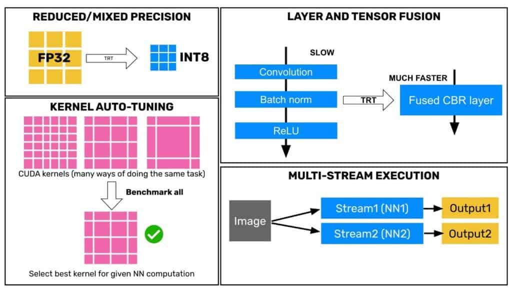
After a neural network has been trained, we can optimize the computational graph for speed (both throughput and latency) at runtime. TensorRT is NVIDIA’s library for optimizing computational graphs for inference on their products.
The job of TensorRT is to take a pre-trained model and ‘compile’ it into an ‘engine’ that runs fast. How fast? That depends on the model itself and the settings used for compilation. First, let’s briefly review some of the strategies used by TensorRT to create an optimized engine:
- Reduced mixed-precision: TRT’s most straightforward optimization method is to reduce the size of weights and biases of the network by converting them from float32 used during training to float16 or int8. Moving data around in a GPU is much more expensive than computation, so reducing the data size to be transferred has a significant impact on performance. When using float16, this conversion does not significantly reduce performance, but the engineer must be careful when using int8 precision. We will specify specific advice in a later section on int8 inference.
- Layer fusion: When certain layers (ex. 1×1 Conv layers in the inception module of Google’s Inception net) can be combined to perform mathematically equivalent operations, TRT fuses them into one layer. This horizontal fusion operation can reduce memory footprint and boost throughput. Another type of layer fusion is vertical fusion, where, for example, convolution, batch norm, and ReLU layers can be combined into one CUDA kernel, tremendously boosting throughput.
- Kernel auto-tuning: A GPU performs parallel computations in a large number of tiny snippets of instructions called kernels. People with experience in CUDA programming know that tuning the parameters of the kernels (most commonly block size, the number of threads in a block, memory management, caching, etc.) can significantly impact the performance of the computational workload. TensorRT does all this for us automatically. Optimally tuned parameters depend on the specific micro-architecture of the hardware. NVIDIA releases kernel tuning guides to port an application from old GPU architectures (like Pascal) to newer ones (like Volta or Ampere). TensorRT takes away all the hassle of figuring out such low-level details of your hardware and gives you the best performance possible on the device you are using.
- Buffer reuse: On embedded systems with low memory, TRT can reuse memory locations corresponding to intermediate outputs of the computation and, therefore, significantly reduce the memory footprint of the network at runtime. This allows large networks, which would not fit into memory, to run in real-time on embedded devices.
- Multi-stream execution: When you have more than one network or multiple copies of the same network or multiple “execution contexts” (we will introduce the term shortly) of one network that you want to infer on, TensorRT, just like CUDA, allows you to run inferences asynchronously on multiple “streams.” This can boost throughput by increasing occupancy of the warps (this is a CUDA concept, don’t worry if you don’t understand it now) on the GPU.
4. Introduction to TensorRT API concepts
Let’s understand how TensorRT’s API is organized. Once you know some key concepts, you will find TensorRT very easy. The concepts are shown in the figure below. Please go through the figure once before reading the explanation and once after.

- Engine: The central object of our attention when using TensorRT is an “engine.” Most of the code we will see will be aimed at either building the engine or using it to perform inference. A TensorRT engine is an object which contains a list of instructions for the GPU to follow. At its core, the engine is a highly optimized computation graph for the GPU (or DLA) that it’s running on. Given an input tensor, the engine tells the GPU what operations to perform to get the neural network’s output.
- Builder: We need to build the engine to use it, so TRT provides a handy ‘builder’ class.
- Builder configuration: The builder needs to know what optimizations to apply while building the engine. For example, you may want to build an engine for INT8 or float16 or even float32 precision. Further, you may wish the engine to execute on GPU or DLA. All these options are specified in a build configuration object.
- Calibrator: Additionally, specifically for INT8 precision, the builder needs additional information, which is provided by a ‘calibrator’ class object. We will explain the role of the calibrator in more detail in the next section.
- Execution stream: The last concept of importance is a stream. A computational stream is a CUDA concept. Typically, CUDA computational workloads are run in streams. Think of a stream like a scope in programming. We know that only variables defined in a scope are accessible to other functions within that scope. For example, a scope makes sure that a variable defined internally within function f will typically not be accessible in another function g. Streams in TensorRT (and VPI, but that’s for another day) provide an excellent way to wrap computation into silos that are not visible to each other. Streams allow us to perform computations asynchronously (out of sequence) even while using a language like Python, in which programs are executed sequentially. We will show an illustrative example of the power of asynchronous execution by showing how to double the inference throughput by using two DLAs simultaneously.
5. Semantic segmentation
Let’s use a concrete example to solidify these concepts. We will take a pre-trained semantic segmentation model from PyTorch’s torchvision library and explore the various ways to accelerate inference of this model using TensorRT on Jetson Xavier AGX.
Torchvision is a library from the creators of PyTorch. It contains a rich collection of many state-of-the-art neural networks for computer vision. We will use a Fully Convolutional Network (FCN) with a ResNet50 backbone.
Introduced by Shelhamer et al. in “Fully Convolutional Networks for Semantic Segmentation”, FCN is a straightforward architecture that uses just convolution, transposed convolution, and max-pooling layers along with skip connections to tackle the problem of semantic segmentation with great success. Though it is not state-of-the-art on benchmarks anymore (Transformers have usurped the throne recently), FCN remains popular in academia and industry because of its outstanding performance on real-world computer vision problems.
This model is an excellent choice for demonstration because, as we will see, the model is somewhat heavy for real-time inference on an embedded board like Jetson AGX but not so heavy that there is no hope at all. As it turns out, this is the territory for most computer vision applications in the industry where you quite often want to run large and expressive models to solve complex problems but not so large models that they cannot run at all. It is, for example, possible to train an FCN model with a lighter backbone like ResNet18. However, given enough data, a ResNet50 backbone would be preferred as deeper models usually achieve better accuracy.
Torchvision provides a simple interface to the FCNResNet50 model pre-trained on the MS COCO dataset (specifically, train2017 subset). The dataset has 20 classes, and along with one background class, the network classifies each pixel of an input image into one of 21 classes.
We will apply the following normalization steps to all input images
- Convert to floating point: We first convert the 8-bit unsigned integer images with range 0-255 to a range between 0 and 1 in floating-point representation.
- Mean subtraction: Next, we subtract the mean value from each channel (0.485 for red, 0.456 for green, and 0.406 for blue channel).
- Divide by standard deviation: Finally, we divide the resulting value by a standard deviation (0.229 for red, 0.224 for green, and 0.225 for blue channel).
The above normalization procedure was used during training, and we will stick to it to make sure that the network sees the same range of inputs as it was trained on.
import torch
from torch import nn
from torchvision import models
import torchvision.transforms as T
import numpy as np
import cv2
import time
from segcolors import colors

class SegModel(nn.Module):
    def __init__(self):
        super().__init__()
        self.net= models.segmentation.fcn_resnet50(pretrained=True, aux_loss=False).cuda()
        self.ppmean=torch.Tensor([0.485, 0.456, 0.406])
        self.ppstd=torch.Tensor([0.229, 0.224, 0.225])
        self.preprocessor=T.Compose([T.ToTensor(), T.Normalize(mean=[0.485, 0.456, 0.406], std = [0.229, 0.224, 0.225])])
        self.cmap=torch.from_numpy(colors[:,::-1].copy())

    def forward(self, x):
        """x is a pytorch tensor"""

        #x=(x-self.ppmean)/self.ppstd #uncomment if you want onnx to include pre-processing
        isize=x.shape[-2:]
        x=self.net.backbone(x)['out']
        x=self.net.classifier(x)
        #x=nn.functional.interpolate(x, isize, mode='bilinear') #uncomment if you want onnx to include interpolation
        return x

    def export_onnx(self, onnxpath):
        """onnxpath: string, path of output onnx file"""

        x=torch.randn(1,3,360,640).cuda() #360p size
        input=['image']
        output=['probabilities']
        torch.onnx.export(self, x, onnxpath, verbose=False, input_names=input, output_names=output, opset_version=11)
        print('Exported to onnx')

    def infervideo(self, fname, view=True, savepath=None):
        """
        fname: path of input video file/camera index
        view(bool): whether or not to display results
        savepath (string or None): if path specified, output video is saved
        """
        src=cv2.VideoCapture(fname)
        ret,frame=src.read()

        if not ret:
            print(f'Cannot read input file/camera {fname}')
            quit()

        self.net.eval()

        dst=None
        fps=0.0

        if savepath is not None:
            dst=self.getvideowriter(savepath, src)

        with torch.no_grad(): #we just inferring, no need to calculate gradients
            while ret:
                outf, cfps=self.inferframe(frame, benchmark=True)
                if view:
                    cv2.imshow('segmentation', outf)
                    k=cv2.waitKey(1)
                    if k==ord('q'):
                        break
                if dst:
                    dst.write(outf)

                fps=0.9*fps+0.1*cfps
                print(fps)
                ret,frame=src.read()

            src.release()
            if dst:
                dst.release()

    def inferframe(self, frame, benchmark=True):
        """
        frame: numpy array containing un-pre-processed video frame (dtype is uint8)
        benchamrk: bool, whether or not to calculate inference time
        """
        rgb=frame[...,::-1].copy()
        processed=self.preprocessor(rgb)[None]
        start, end = 1e6, 0

        if benchmark:
            start=time.time()

        processed=processed.cuda() #transfer to GPU <-- does not use zero copy
        inferred= self(processed) #infer

        if benchmark:
            end=time.time()

        inferred=inferred.argmax(dim=1)

        overlaid=self.overlay(frame, inferred)
        return overlaid, 1.0/(end-start)

    def overlay(self, bgr, mask):
        """
        overlay pixel-wise predictions on input frame
        bgr: (numpy array) original video frame read from video/camera
        mask: (numpy array) class mask containing one of 21 classes for each pixel
        """
        colored = self.cmap[mask].to('cpu').numpy()[0,...]
        colored=cv2.resize(colored, (bgr.shape[1], bgr.shape[0]), interpolation=cv2.INTER_CUBIC)
        oved = cv2.addWeighted(bgr, 0.7, colored, 0.3, 0.0)
        return oved

    def getvideowriter(self, savepath, srch):
        """
        Simple utility function for getting video writer
        savepath: string, path of output file
        src: a cv2.VideoCapture object
        """
        fps=srch.get(cv2.CAP_PROP_FPS)
        width=int(srch.get(cv2.CAP_PROP_FRAME_WIDTH))
        height=int(srch.get(cv2.CAP_PROP_FRAME_HEIGHT))
        fourcc=int(srch.get(cv2.CAP_PROP_FOURCC))
        dst=cv2.VideoWriter(savepath, fourcc, fps, (width, height))
        return dst

if __name__=='__main__':
    model=SegModel()
    model.export_onnx('./segmodel.onnx')
5.1 Understanding inference metrics and measuring performance
As explained in the previous section, we can use the script above to evaluate the inference throughput of this model using PyTorch as a baseline. Using the latest (as of the time of writing) JetPack version 4.6 (rev. 3) and PyTorch 1.9.0, we achieved ~6 fps using torch CUDA with an input size of 640 pixels x 360 pixels. This corresponds to a latency of about 160 milliseconds for a batch size of 1. This means that a minimum of 160 milliseconds is required for processing one image. It is possible to process multiple images simultaneously by batching them into one input tensor and getting multiple outputs within the same period. This is called throughput, and batching is essential for cloud-based applications where hundreds of API calls might be made by various devices to the server simultaneously. However, for robotics applications with an embedded processor, there are usually just 1 or 2 sources of inputs (say a pair of stereo cameras). In such cases, throughput at batch size 1 or 2 is most important. When evaluating systems/software/hardware or tools for robotics, it’s important to remember this distinction and not get confused or misled by a vendor’s claims. For this blog post, we will evaluate all methods for batch size 1. In this case, the throughput is just 1/latency.
So, with this understanding, we realize that the throughput of 6 fps is grossly insufficient for a real-time system where the camera is usually streaming data at 30 frames per second. Another issue is that to achieve the 6 fps; we use almost all the GPU resources available. Usually, a deep learning model is a part of the perception software stack of the robot. It is common to have multiple computationally expensive algorithms running within the perception stack. For example, Simultaneous Localization and Mapping (SLAM) is commonly used in robotics and often runs alongside other perception tasks. Apart from perception, the equally important navigation stack might be running a path planning algorithm that might also contend for the system’s resources. Can TensorRT help us spread the workload and alleviate the load on the GPU? Yes!
5.2 Constructing the computation engine in Python with TensorRT API
Having understood the limitations of a framework like PyTorch for real-time inference, we will now switch to TRT and show how to use TRT for squeezing every bit of performance that the hardware is capable of. The first step in accelerating a neural network in TensorRT is creating the engine. To create an engine from a pre-trained model, we first declare a builder object (called builder in code) and a network object (referred to as net in the code). We use an ONNX parser to read the specifications of the network and populate the net object with layers. The net object is internal to TensorRT and is not used for inference.
Once the net object contains layers from the pre-trained model, we need to tell the builder what precision we want the engine to support and what devices the engine should run on (remember there are two DLAs on the Jetson apart from GPU, which can also be used for inference). For example, TensorRT supports float32, float16, and int8 precisions. GPU and DLA (DLA0 and DLA1) devices are supported. These options are wrapped neatly in a build configuration object (called config in the code). Specifying the precision and device in the config is very easy by just setting some flags.
def parse_or_load(self): #method of TRTSegmentor object
		logger= trt.Logger(trt.Logger.INFO)
		#we want to show logs of type info and above (warnings, errors)

		if os.path.exists(self.enginepath):
			logger.log(trt.Logger.INFO, 'Found pre-existing engine file')
			with open(self.enginepath, 'rb') as f:
				rt=trt.Runtime(logger)
				engine=rt.deserialize_cuda_engine(f.read())

			return engine, logger

		else: #parse and build if no engine found
			with trt.Builder(logger) as builder:
				builder.max_batch_size=self.max_batch_size
				#setting max_batch_size isn't strictly necessary in this case
				#since the onnx file already has that info, but its a good practice

				network_flag = 1 << int(trt.NetworkDefinitionCreationFlag.EXPLICIT_BATCH)

				#since the onnx file was exported with an explicit batch dim,
				#we need to tell this to the builder. We do that with EXPLICIT_BATCH flag

				with builder.create_network(network_flag) as net:

					with trt.OnnxParser(net, logger) as p:
						#create onnx parser which will read onnx file and
						#populate the network object `net`
						with open(self.onnxpath, 'rb') as f:
							if not p.parse(f.read()):
								for err in range(p.num_errors):
									print(p.get_error(err))
							else:
								logger.log(trt.Logger.INFO, 'Onnx file parsed successfully')

						net.get_input(0).dtype=trt.DataType.HALF
						net.get_output(0).dtype=trt.DataType.HALF
						#we set the inputs and outputs to be float16 type to enable
						#maximum fp16 acceleration. Also helps for int8

						config=builder.create_builder_config()
						#we specify all the important parameters like precision,
						#device type, fallback in config object

						config.max_workspace_size = self.maxworkspace

						if self.precision_str in ['FP16', 'INT8']:
							config.flags = ((1<<self.precision)|(1<<self.allowGPUFallback))
							config.DLA_core=self.dla_core
						# DLA core (0 or 1 for Jetson AGX/NX/Orin) to be used must be
						# specified at engine build time. An engine built for DLA0 will
						# not work on DLA1. As such, to use two DLA engines simultaneously,
						# we must build two different engines.

						config.default_device_type=self.device
						#if device is set to GPU, DLA_core has no effect

						config.profiling_verbosity = trt.ProfilingVerbosity.VERBOSE
						#building with verbose profiling helps debug the engine if there are
						#errors in inference output. Does not impact throughput.

						if self.precision_str=='INT8' and self.calibrator is None:
							logger.log(trt.Logger.ERROR, 'Please provide calibrator')
							#can't proceed without a calibrator
							quit()
						elif self.precision_str=='INT8' and self.calibrator is not None:
							config.int8_calibrator=self.calibrator
							logger.log(trt.Logger.INFO, 'Using INT8 calibrator provided by user')

						logger.log(trt.Logger.INFO, 'Checking if network is supported...')

						if builder.is_network_supported(net, config):
							logger.log(trt.Logger.INFO, 'Network is supported')
							#tensorRT engine can be built only if all ops in network are supported.
							#If ops are not supported, build will fail. In this case, consider using
							#torch-tensorrt integration. We might do a blog post on this in the future.
						else:
							logger.log(trt.Logger.ERROR, 'Network contains operations that are not supported by TensorRT')
							logger.log(trt.Logger.ERROR, 'QUITTING because network is not supported')
							quit()

						if self.device==trt.DeviceType.DLA:
							dla_supported=0
							logger.log(trt.Logger.INFO, 'Number of layers in network: {}'.format(net.num_layers))
							for idx in range(net.num_layers):
								if config.can_run_on_DLA(net.get_layer(idx)):
									dla_supported+=1

							logger.log(trt.Logger.INFO, f'{dla_supported} of {net.num_layers} layers are supported on DLA')

						logger.log(trt.Logger.INFO, 'Building inference engine...')
						engine=builder.build_engine(net, config)
						#this will take some time

						logger.log(trt.Logger.INFO, 'Inference engine built successfully')

						with open(self.enginepath, 'wb') as s:
							s.write(engine.serialize())
						logger.log(trt.Logger.INFO, f'Inference engine saved to {self.enginepath}')

		return engine, logger
5.3 Int8 precision and calibration
However, things are a little bit more involved for int8 precision. As explained very nicely in one of our earlier blog posts, int8 precision requires converting the floating-point parameters of the network into 8-bit integers. Since the dynamic range of floating-point numbers is much larger than 8-bit integers, the conversion needs to be done carefully to avoid a huge reduction in accuracy. This process of carefully converting parameters from floating-point into integer type with minimum loss in accuracy is called calibration. There are several algorithms for calibration, and here is an excellent survey of some popular ones. Luckily, we don’t have to know any of the details of calibration algorithms to use them. TensorRT provides a calibrator class to help us in this process. The calibrator class feeds some example images of the type that the network is expected to see during inference, and based on the range of activations, TensorRT figures out how to calibrate the int8 parameters. Many popular calibration algorithms are implemented, and we can just subclass them to create our own calibrator.
Here, we will subclass the Int8EntropyCalibrator2 class. Since the calibration algorithm is already implemented, we simply tell the calibrator how to get batches for the inference to run. This is done by overriding the get_batch function of the calibrator class. During calibration, the calibrator goes through every image in the dataset and runs inference on it. This can take a long time, so TensorRT provides us a way to save intermediate results of the process in a cache file so that if we need to build the engine again in int8, we can save a lot of time. We override the read_calibration_cache and write_calibration_cache functions to tell the calibrator where to store the cache file. It is highly recommended to save the cache as it will save you a lot of time. Finally, note that we should provide the calibrator with a set of example images. NVIDIA recommends providing about 500 images for good calibration. We will use images from the COCO validation set, which contains 5000 images. Now, let’s dive into the code.
6. Creating inference pipeline
The final piece of the puzzle that we need to assemble before starting inference is a buffer. A buffer is just a blob of memory allocated for the inputs and outputs of the engine. We use the python interface for CUDA, called PyCUDA, to allocate memory to hold our inputs and outputs. Once the memory is allocated, we transfer the input data from a NumPy array to the CUDA buffer using a PyCUDA function. After that, we just call the execute function on the engine stream, and the TensorRT engine will perform inference. The output will be stored in the output buffer we allocated earlier. We transfer the output data to a NumPy array using another PyCUDA function, and that’s it, we have the inference output ready to use in a NumPy array format. Let us see how these things fit together in code.
def preprocess(self, img): #preprocessing images
		img=cv2.resize(img,(self.in_w,self.in_h))
		img=img[...,::-1]
		img=img.astype(np.float32)/255
		img=(img-self.pp_mean)/self.pp_stdev

		img=np.transpose(img,(2,0,1))
		img=np.ascontiguousarray(img[None,...]).astype(self.dtype)

		return img

def infer(self, image, benchmark=False): #method of TRTSgmentor class
		"""
		image: unresized,
		"""
		intensor=self.preprocess(image)

		start=time.time()

		cuda.memcpy_htod_async(self.d_input, intensor, self.stream)
		self.context.execute_async_v2(self.bindings, self.stream.handle, None)
		cuda.memcpy_dtoh_async(self.output, self.d_output, self.stream)

		self.stream.synchronize()

		if benchmark:
			duration=(time.time()-start)
			return duration
Now that we have created an object that can perform inference on either GPU or DLA, we can use it as an abstraction for performing inference on 2 DLAs in parallel.
def infervideo_2DLAs(infile, onnxpath, calibrator=None, precision='INT8',display=False):
	src=cv2.VideoCapture(infile)
	seg1=TRTSegmentor(onnxpath, colors, device='DLA', precision=precision ,calibrator=calibrator, dla_core=0)
	seg2=TRTSegmentor(onnxpath, colors, device='DLA', precision=precision ,calibrator=calibrator, dla_core=1)
	ret1,frame1=src.read()
	ret2,frame2=src.read()
	fps=0.0

	while ret1 and ret2:
		intensor1=seg1.preprocess(frame1)
		intensor2=seg2.preprocess(frame2)

		start=time.time()

		cuda.memcpy_htod_async(seg1.d_input, intensor1, seg1.stream)
		cuda.memcpy_htod_async(seg2.d_input, intensor2, seg2.stream)

		seg1.context.execute_async_v2(seg1.bindings, seg1.stream.handle, None)
		seg2.context.execute_async_v2(seg2.bindings, seg2.stream.handle, None)

		cuda.memcpy_dtoh_async(seg1.output, seg1.d_output, seg1.stream)
		cuda.memcpy_dtoh_async(seg2.output, seg2.d_output, seg2.stream)

		seg1.stream.synchronize()
		seg2.stream.synchronize()

		end=time.time()
		if display:
			drawn1=seg1.draw(frame1)
			drawn2=seg2.draw(frame2)
			cv2.imshow('segmented1', drawn1)
			cv2.imshow('segmented2', drawn2)
			k=cv2.waitKey(1)
			if k==ord('q'):
				break

		fps=0.9*fps+0.1*(2.0/(end-start))
		print('FPS = {:.3f}'.format(fps))

		ret1,frame1=src.read()
		ret2,frame2=src.read()
7. Results
Now that we can run the inference script with various command-line options.
Here is how to run fp16 inference on a stored video:
python3 pytrt.py --precision fp16 --device gpu --infile input.mp4
Similarly, you can run inference in int8 format with
python3 pytrt.py --precision int8 --device gpu --infile input.mp4
If you want to use the DLA, just change the device type to DLA as:
python3 pytrt.py --precision fp16 --device dla --infile input.mp4
Or
python3 pytrt.py --precision int8 --device dla --infile input.mp4
To run inference on DLA with int8 precision. Note that DLA does not support fp32 inference.
As a baseline, you can also run inference on the GPU at fp32 precision with
python3 pytrt.py --precision fp32 --device gpu --infile input.mp4
The script will perform inference and show the inference throughput in fps for batch size 1.
7.1 How do I know if DLA is really being used?
Since DLA’s support a limited set of layers, it is quite common for the GPU to be partly used when an engine is complied for DLA. It is desirable to verify and benchmark exactly how much of the DLA’s resources are being used in such cases. Popular tools like top, htop, and even jtop don’t provide a way to measure the use of DLAs. The usage statistics about DLA are stored in the `/sys` directory of the Linux operating system in certain files. These files are updated very frequently (this should all sound familiar if you know how everything in Linux is a file, including something like a printer device).
Therefore, to measure DLA usage, we can just read these files with a Shell script and get descriptors such as –
- The DLA is enabled or disabled.
- The DLA is active or inactive. The DLA automatically becomes inactive while not in use, even if it is enabled,
- Usage status. It is a number between 0 and 10, with 10 representing 100% usage. Here is a shell script for reading all the data available about DLA.
device="dla"

if [[ !($1 = "") ]]
then

device=$1

fi

if [[ $device = "dla" ]]

then

export dev0_name="DLA 0"
export dev0_dir="15880000.nvdla0"
export dev1_name="DLA 1"
export dev1_dir="158c0000.nvdla1"

else

export dev0_name="PVA 0"
export dev0_dir="16000000.pva0"
export dev1_name="PVA 1"
export dev1_dir="16800000.pva1"
fi

echo $dev0_name
echo "Enabled: $(cat /sys/devices/platform/host1x/$dev0_dir/power/runtime_enabled)"
echo "Control: $(cat /sys/devices/platform/host1x/$dev0_dir/power/control)"
echo "Status: $(cat /sys/devices/platform/host1x/$dev0_dir/power/runtime_status)"
echo "Usage: $(cat /sys/devices/platform/host1x/$dev0_dir/power/runtime_usage)"

echo ""

echo $dev1_name
echo "Enabled: $(cat /sys/devices/platform/host1x/$dev1_dir/power/runtime_enabled)"
echo "Control: $(cat /sys/devices/platform/host1x/$dev1_dir/power/control)"
echo "Status: $(cat /sys/devices/platform/host1x/$dev1_dir/power/runtime_status)"
echo "Usage: $(cat /sys/devices/platform/host1x/$dev1_dir/power/runtime_usage)"
You should open a new console to use this script and run it as:
watch -n 1 bash check_dla_pva_usage.sh
Here is a screenshot of a typical output might get while using both DLAs for inference:
Now that we know how to use TensorRT and monitor system usage, we can run an inference with various configurations described above and analyze the results. Here are the results I got on JAX running the latest JetPack 4.6 rev 3 for an input image size of 640 pixels x 360 pixels:
As we saw earlier, the GPU is painfully slow when executing at fp32 and well below the throughput required for the real-time performance of 30 fps. Just changing the precision to fp16 dramatically improves performance on the GPU and we now run at 32 fps which is already faster than real-time. You can also get a similar speedup in PyTorch by calling `net.half()` on the network and input tensors. However, TensorRT allows us to go much beyond that.
By using int8 calibration, we almost double (!) the throughput again to 59 fps on this pretty heavy model, which means that the GPU becomes free to run other computational workloads. Note that this is 10x the throughput of the original model. But that’s not all. By simply changing the device parameter in the code, we can run the network on DLA (with GPU fallback on some layers).
As it turns out, the network is too heavy for a single DLA to run in real-time, even at int8 precision. We obtain 11 fps at fp16 and 21 fps at int8 precision. Now, since we have two DLAs in the JAX system, we can combine them to almost double the throughput again. We double the inference throughput to about 38 fps using this simple trick. Using TRT enables us to perform inference faster than in real-time with very minimal use of the GPU. The GPU is genuinely free, and we get much more breathing room for designing other parts of our computer vision application.
We chose an off-the-shelf network from a popular deep learning library for this blog post. As it turns out, some layers of this network can’t run on the DLA, but now that you have learned how to use TRT. As a computer vision engineer trying to solve real-world problems, you have learned to benchmark various architectures for your application and choose one that can run entirely on the DLA(s) and leave the GPU completely free.
8. Summary
This blog post is very different from our usual content. We have taken a step back from learning about ever more sophisticated deep learning algorithms, and we have stepped into the world of industrial-grade, production-ready computer vision applications. We first discovered the unique requirements of industrial computer vision and how it differs from research and proofs of concept. We then briefly reviewed the features of one of the leading edge devices for industrial deep learning solutions, NVIDIA’s Jetson AGX.
Next, we delved into the concepts of TensorRT and learned how these concepts fit together to allow us to accelerate deep learning inference on edge devices. We solidified these concepts with the example of a semantic segmentation network from PyTorch’s torchvision library. We learned how to use PyCUDA to interface between python’s NumPy array and CUDA buffer. We also learned how to use int8 precision on the Jetson along with DLA and measure DLA performance and usage.
The results were impressive. We could increase the inference throughput by about 10x compared to naive PyTorch (fp32) implementation on the GPU. We also found ways of using the two DLAs in clever ways to achieve faster than real-time performance with minimal use of the GPU. These results underscore the importance of optimization in deploying deep learning models and why every computer vision engineer should be familiar with TensorRT. We are just getting started with building industrial-grade computer vision, so please stay tuned.
References:
- https://www.daxx.com/blog/development-trends/c-automotive
- https://ieeexplore.ieee.org/document/8479057
- ISO26262 For Software Developers https://incoseil.org › check_download_nopass › fi…
- https://www.whitesourcesoftware.com/resources/blog/open-source-licenses-explained/
- https://www.fierceelectronics.com/electronics/nvidia-has-80-share-ai-processors-omdia-says-except
- https://www.anandtech.com/show/13584/nvidia-xavier-agx-hands-on-carmel-and-more/3
- https://en.wikipedia.org/wiki/Project_Denver
- https://www.anandtech.com/show/13584/nvidia-xavier-agx-hands-on-carmel-and-more
- https://developer.nvidia.com/blog/nvidia-jetson-agx-xavier-32-teraops-ai-robotics/?ncid=so-fac-mdjngxxrmllhml-69163
- https://developer.nvidia.com/embedded/jetson-agx-xavier-developer-kit








100K+ Learners
Join Free OpenCV Bootcamp3 Hours of Learning