Introduction
Image classification is a key task in Computer Vision.
In an image classification task, the input is an image, and the output is a class label (e.g. “cat”, “dog”, etc. ) that usually describes the content of the image.
In the last decade, neural networks have made great progress in solving the image classification task. The application of neural networks to the classification problem started in 2012 with the introduction of AlexNet by Alex Krizhevsky, Ilya Sutskever, and Geoffrey Hinton. Their model achieved 63.3% Top-1 Accuracy on the ImageNet challenge. Currently, the Top-1 result (as of August 2020) is 88.5% achieved by the network called “FixEfficientNet-L2.”

The task of assigning a label to a picture is well studied. Often it’s enough to search on GitHub for a model (or implement it by yourself) and train it on your data. You get a solution that can predict the labels with decent accuracy.
However, when you aren’t satisfied with the result, improving the model may be tricky. You can try to one of the following.
- Use another model. For instance, if you work with the ResNet family, you may try to use a larger model or switch to one of the more recent modifications like ResNeSt. However, this isn’t always possible as you may be limited in resources (for example if your target is a small device like Raspberry Pi), the state-of-the-art model with hundreds of millions of parameters may not fit into memory, or inference may be too slow. Moreover, usually, we use transfer learning from pre-trained models, you need to find weights for your model but if you make some custom updates or find a model on GitHub it can be an issue. That is why sometimes you have to fix the chosen model and find other ways to improve quality.
- Increase the dataset size. Often adding extra samples may boost the quality. It’s an obvious option and it really may help the model to generalize better but there are some issues. First of all, you need to label the new data or find a well-labeled public dataset. In the classification task, labeling is usually considered to be simple but this depends heavily on the task specifics. For example, medical images may be hard to acquire and even harder to label. Also, you need to make sure that this new data will have a similar distribution and won’t mess with the model.
- Fine-tune the hyperparameters. The neural network updates millions of parameters by itself but there are several hyperparameters such as optimizer parameters, loss weights, etc. which should be found by the researcher. As there are plenty of possible combinations of hyper-parameters, it may be hard to find the best one without any prior knowledge or intuition.
- Use some “tricks.” They are the best practices which people resort to improve performance. These tricks are different from hyperparameters tuning as you need to understand what’s happening inside your model and during the training process. By updating some parameters during training (for example using a specific learning rate scheduler) or during model weight initialization in a specific way you can make the training more stable and improve the result.
Today we’re going to use the last option and try to boost the model performance by applying the methods which were tested by Tong He, Zhi Zhang Hang Zhang, et al. in their survey “Bag of Tricks for Image Classification with Convolutional Neural Networks”.
Dataset
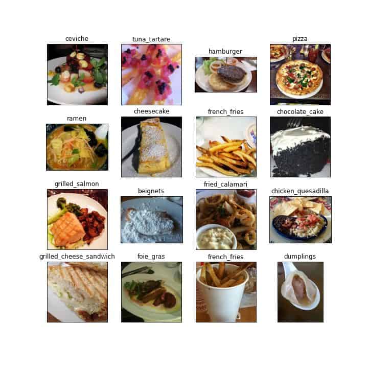
In our experiments, we’re going to use Food-101 Dataset. It is available on Kaggle.
The dataset was introduced in Food-101 – Mining Discriminative Components with Random Forests by Lukas Bossard, Matthieu Guillaumin, and Luc Van Gool.
It includes 101 classes of food. Each class contains 1000 images. Therefore, the whole dataset includes 101,000 images and is divided into train and test subsets. The train part consists of 750 images for each class. However, to increase training speed, we reduced the number of classes from 101 to 21.
Please, follow the instruction to prepare the dataset:
- Download zip-archive from Kaggle;
- Unzip the data;
- Use
split_food-101.pyto split Food-101 into train/test folders. This script will parsetrain.txtandtest.txtand copy images into corresponding sub-folders. Note that we hard-coded the classes which we are going to use.
Baseline
We used ResNet-18 architecture as a baseline. To improve the results, we used a pre-trained on the ImageNet model with Adam optimizer and CrossEntropy loss function. Default LR was ![]() , which was multiplied with gamma 0.1, following MultiStepLR Policy, after epochs 15 and 30. Overall the model was trained for 40 epochs on 1 Nvidia 1080Ti GPU with the batch size equal to 32. We also used the PyTorch-Lightning framework as a wrapper to organize our code. We have several posts about this framework (Getting Started with PyTorch Lightning and TensorBoard with PyTorch Lightning), which can make you familiar with it.
, which was multiplied with gamma 0.1, following MultiStepLR Policy, after epochs 15 and 30. Overall the model was trained for 40 epochs on 1 Nvidia 1080Ti GPU with the batch size equal to 32. We also used the PyTorch-Lightning framework as a wrapper to organize our code. We have several posts about this framework (Getting Started with PyTorch Lightning and TensorBoard with PyTorch Lightning), which can make you familiar with it.
Note: To make our results more reliable, we launch every experiment 3 times with different seeds and provide the mean result.
As our dataset is large and varied, we use a straightforward augmentation policy. During training we used:
- RandomResizedCrop;
- HorizontalFlip;
- Normalization;
def get_training_augmentation():
    augmentations_train = A.Compose(
        [
            A.RandomResizedCrop(224, 224, scale=(0.8, 1.0)),
            A.HorizontalFlip(),
            A.Normalize(mean=[0.485, 0.456, 0.406], std=[0.229, 0.224, 0.225]),
            ToTensorV2(),
        ],
    )
    return lambda img: augmentations_train(image=np.array(img))
During validation, we follow the authors’ strategy and resize the shorter side of the image to 256, keeping the aspect ratio. After that, we applied center crop to get 224×224 square:
def get_test_augmentation():
    augmentations_val = A.Compose(
        [
            A.SmallestMaxSize(256),
            A.CenterCrop(224, 224),
            A.Normalize(mean=[0.485, 0.456, 0.406], std=[0.229, 0.224, 0.225]),
            ToTensorV2(),
        ],
    )
    return lambda img: augmentations_val(image=np.array(img))
Tricks for Image Classification
To begin with, let’s split up our tricks into two categories:
- Efficient Training Tricks – hardware and model connected tricks which can possibly improve the performance;
- Training Refinements – several interesting approaches for further quality improvement.
Let’s discuss each trick in detail.
Efficient Training Tricks
Trick #1: Large Batch Training
Batch size is a crucial training parameter, and, even though it seems obvious that the larger batch size will result in faster convergence and better results, one can find different opinions about its optimal value. It is controversial and, at the same time, a well-studied topic. You can find research about small versus large batch size tradeoff on Medium. Also, you can read about the impact of batch size on the variance of gradients here. Below are some heuristics to deal with this issue. As we are limited in resources, we experimented with batch sizes 16, 32, 64, 96.
When we increase the batch size, we don’t change the expectation of the stochastic gradient, but reduce the noise and, therefore, reduce the variance. It means that with larger batches we could use a greater learning rate. One of the popular approaches is to linearly scale the learning rate during training. For instance, let’s assume we choose ![]() as an initial learning rate for batch size 32. Then, by changing the batch size value to
as an initial learning rate for batch size 32. Then, by changing the batch size value to ![]() , we increase the learning rate to
, we increase the learning rate to ![]() . However, we empirically found that in our case, Adam optimizer with the learning rate
. However, we empirically found that in our case, Adam optimizer with the learning rate ![]() leads to better convergence and stability, so we didn’t experiment with linear scaling much.
leads to better convergence and stability, so we didn’t experiment with linear scaling much.
| Experiment | Batch Size | Top-1 Accuracy | STD | Training Time |
|---|---|---|---|---|
| Baseline | 32 | 90.21% | 0.18% | 43m |
| BS16 | 16 | 90.21% | 0.35% | 45m |
| BS64 | 64 | 90.14% | 0.16% | 33m |
| BS96 | 96 | 89.81% | 0.13% | 32m |
The larger the batch size we use, the lower the training time and accuracy value are.
Trick #2: LR Warm-up
Following this heuristic, we use the first few epochs to “warm-up” the learning rate. Using a higher learning rate at the beginning of training (when all the parameters are far away from the optimal ones) may lead to lower quality due to the appearance of numerical instability. Assume we want to warm-up during the first ![]() epochs with the initial learning rate
epochs with the initial learning rate ![]() , then at epoch
, then at epoch ![]() ,
, ![]() , the learning rate is calculated as
, the learning rate is calculated as ![]() :
:
def optimizer_step(self, epoch, batch_idx, optimizer, *args, **kwargs):
    # Learning Rate warm-up
    if self.args.warmup != -1 and epoch < self.args.warmup:
        lr = self.args.lr * (epoch + 1) / self.args.warmup
        for pg in optimizer.param_groups:
            pg["lr"] = lr
After that, we can follow any strategy (multi-step decay, reduce on the plateau). In our experiments, we used 6 epochs for warm-up, until the learning rate became ![]() , and then it was reduced to
, and then it was reduced to ![]() ,
, ![]() on epochs 15 and 30 correspondingly.
on epochs 15 and 30 correspondingly.

Overall, this trick improved the quality by 0.08% which is not very significant.
| Experiment | Batch Size | LR Warmup | Mean Accuracy | STD |
|---|---|---|---|---|
| Baseline | 32 | No | 90.21% | 0.18% |
| Warm-up | 32 | Yes | 90.29% | 0.02% |
Trick #3: Mixed Precision operations
With the help of common frameworks (PyTorch, TensorFlow) we train our models in 32-bit floating-point precision format (FP32). In other words, all the parameters, gradients, results of arithmetic operations are stored in this format. However, modern hardware may show better performance on lower precision data types due to optimized logic units. Authors of the article state that their Nvidia V100 offers 14 TFLOPS in FP32 but 100 TFLOPS in FP16. Unfortunately, our GPU (Nvidia 1080Ti) has low-rate FP16 performance so we won’t see any significant difference in FP32 and FP16 performances. You can follow the link for more details about mixed-precision training.
| Experiment | Batch Size | Precision | Top-1 Accuracy | STD | Training Time |
|---|---|---|---|---|---|
| Baseline | 32 | FP32 | 90.21% | 0.18% | 43m |
| FP16 | 32 | FP16 | 90.36% | 0.11% | 35m |
| BS16, FP16 | 16 | FP16 | 90.25% | 0.30% | 38m |
| BS64, FP16 | 64 | FP16 | 90.20% | 0.03% | 30m |
| BS96, FP16 | 96 | FP16 | 89.78% | 0.19% | 29m |
As you can see, FP16 improved training speed for all of the batch size (BS) settings, but there was also an accuracy increase. We used the Nvidia apex library with the O0 optimization level for FP32 and O1 for FP16. Follow the link for details. PyTorch-Lightning allows you to switch between FP32 and FP16 easily by adding --amp_level [Opt_level] key into command line arguments.
Training Refinements
Trick #4: Cosine LR Decay
Along with the multi-step decay learning rate policy, there are a couple more policies that we could use. For instance, we can apply a cosine function to decrease the learning rate from the initial value to 0. If we have ![]() epochs (warmup stage is ignored) with an initial learning rate
epochs (warmup stage is ignored) with an initial learning rate ![]() , then at epoch
, then at epoch ![]() , the learning rate
, the learning rate ![]() is computed as:
is computed as:
![]()
The idea is to smoothly decrease the learning rate, which could lead to better training results compared to the step decay policy. In cosine decay, we slowly decrease the learning rate at the beginning and the end, while in the middle, the decrease rate is almost linear.

As could be noticed, in our case, this approach improved the quality. Moreover, the experiment with the cosine strategy was less time-consuming.
| Experiment | Top-1 Accuracy | STD | Training Time |
|---|---|---|---|
| Baseline | 90.21% | 0.18% | 43m |
| Cosine Scheduler | 90.38% | 0.19% | 36m |
Trick #5: Label Smoothing
In image classification, we usually use cross-entropy loss function:
![\[\frac{1}{N}(\sum_{c=1}^{N}{y_ilog(\hat{y_i})}),\]](https://learnopencv.com/wp-content/ql-cache/quicklatex.com-04a8e48a1823c492be20dc15b91a16f9_l3.png)
![]()
![]()
With label smoothing, we replace binary indicators ![]() with:
with:
![\[y_i = \begin{cases} 1 - \epsilon, & \mbox{if } i = y \\ \epsilon / (N-1), & \mbox{otherwise }\end{cases}\]](https://learnopencv.com/wp-content/ql-cache/quicklatex.com-07214d5620366a3fb1adf3d11435cd15_l3.png)
![]()
Code implementation:
# Based on https://github.com/pytorch/pytorch/issues/7455
class LabelSmoothingLoss(nn.Module):
    def __init__(self, n_classes, smoothing=0.0, dim=-1):
        super(LabelSmoothingLoss, self).__init__()
        self.confidence = 1.0 - smoothing
        self.smoothing = smoothing
        self.cls = n_classes
        self.dim = dim

    def forward(self, output, target, *args):
        output = output.log_softmax(dim=self.dim)
        with torch.no_grad():
            # Create matrix with shapes batch_size x n_classes
            true_dist = torch.zeros_like(output)
            # Initialize all elements with epsilon / N - 1
            true_dist.fill_(self.smoothing / (self.cls - 1))
            # Fill correct class for each sample in the batch with 1 - epsilon
            true_dist.scatter_(1, target.data.unsqueeze(1), self.confidence)
        return torch.mean(torch.sum(-true_dist * output, dim=self.dim))
With one-hot encoded targets, the model is usually too confident about its predictions as this approach forces the model to make the largest possible logit gaps. That means that training results will be in a huge difference between the correct class logit and others, while also making it possible for incorrect class logits to be quite different from each other.
The usage of label smoothing encourages the model to produce a finite output from the fully-connected layer, which may lead to better generalization. It forces the model to make differences between the logit of the correct class and others a constant dependent on ![]() .
.
| Experiment | Top-1 Accuracy | STD | Training Time |
|---|---|---|---|
| Baseline | 90.21% | 0.18% | 43m |
| Label Smoothing | 91.05% | 0.27% | 37m |
Overall, label smoothing improved our results by 0.9% and we also decreased training time by 6 minutes.
Trick #6: Knowledge Distillation
The usage of knowledge distillation means training a complex and heavy model (we use ResNet-50), which is called a teacher model, and then train a lighter model (a student model) with the help of the teacher. We assume that a more complex model should show higher quality, so, theoretically, it can boost the results of the student model while preserving its simplicity. The student tries to replicate the results of the teacher.
To provide distillation, we modify the loss function. We penalize the difference between the outputs from the teacher and the student. Our loss function changes from the cross-entropy loss, which we’ve already mentioned, to:
![]()
![]()
![]()
See this report for more details.
Code implementation:
# Based on https://github.com/peterliht/knowledge-distillation-pytorch/blob/master/model/net.py
class KnowledgeDistillationLoss(nn.Module):
    def __init__(self, alpha, T, criterion=nn.CrossEntropyLoss()):
        super().__init__()
        self.criterion = criterion
        self.KLDivLoss = nn.KLDivLoss(reduction="batchmean")
        self.alpha = alpha
        self.T = T

    def forward(self, input, target, teacher_target):
        loss = self.KLDivLoss(
            F.log_softmax(input / self.T, dim=1),
            F.softmax(teacher_target / self.T, dim=1),
        ) * (self.alpha * self.T * self.T) + self.criterion(input, target) * (
            1.0 - self.alpha
        )
        return loss
We used ResNet-50 as a teacher model. The model was trained with label smoothing, cosine annealing LR, and linear warmup and achieved 92.18% Top-1 Accuracy.
| Experiment | Top-1 Accuracy | STD | Training Time |
|---|---|---|---|
| Baseline | 90.21% | 0.18% | 43m |
| Knowledge Distillation | 90.72% | 0.17% | 58m |
We achieved a significant growth in quality but increased training time as we need to get predictions from the teacher.
Trick #7: Mix-up Augmentation
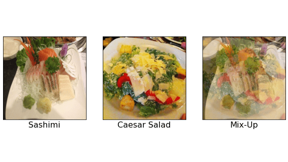
Mix-up is an augmentation technique that constructs a new image as a linear combination of 2 others. Assume we have two batches of samples (we take our current batch and the batch from the earlier iteration), what we do is we randomly shuffle the second one and create a linear combination of images from both batches:
![]()
As targets we take labels from both batches. We calculate loss for each label and return a weighted sum as a total loss:
![]()
There ![]() is a random number drawn from
is a random number drawn from ![]() distribution with hyper-parameter
distribution with hyper-parameter ![]() .
.
Also, it’s possible to make an augmented target for this new sample as a linear combination of original targets (if your targets are one-hot encoded or smoothed).
This trick helps to reduce the number of confident predictions and can boost the quality, but for a human it may be difficult to decide what’s in the augmented picture.
Code implementation:
    def mixup_batch(self, x, y, x_previous, y_previous):
        lmbd = (
            np.random.beta(self.args.mixup_alpha, self.args.mixup_alpha)
            if self.args.mixup_alpha > 0
            else 1
        )
        if x_previous is None:
            x_previous = torch.empty_like(x).copy_(x)
            y_previous = torch.empty_like(y).copy_(y)
        batch_size = x.size(0)
        index = torch.randperm(batch_size)
        # If current batch size != previous batch size, we take only a part of the previous batch
        x_previous = x_previous[:batch_size, ...]
        y_previous = y_previous[:batch_size, ...]
        x_mixed = lmbd * x + (1 - lmbd) * x_previous[index, ...]
        y_a, y_b = y, y_previous[index]
        return x_mixed, y_a, y_b, lmbd

class MixUpAugmentationLoss(nn.Module):
    def __init__(self, criterion):
        super().__init__()
        self.criterion = criterion

    def forward(self, input, target, *args):
        # Validation step
        if isinstance(target, torch.Tensor):
            return self.criterion(input, target, *args)
        target_a, target_b, lmbd = target
        return lmbd * self.criterion(input, target_a, *args) + (
            1 - lmbd
        ) * self.criterion(input, target_b, *args)
The result of applying this technique could be found in the table below:
| Experiment | Top-1 Accuracy | STD | Training Time |
|---|---|---|---|
| Baseline | 90.21% | 0.18% | 43m |
| Mix-Up | 90.66% | 0.26% | 48m |
Mix-up augmentation between two batches with label smoothing improved the quality but took more time.
Bonus: Trick combination
Finally, we combined all the tricks which gave us some boost and launched an experiment with this setup. Overall, we used:
- Linear Warm-Up;
- Cosine Scheduling;
- Label Smoothing;
- Knowledge Distillation;
It could be expected that the combination of the tricks should give us a strong improvement as we combine the best ones. This setup led to some growth. Overall, we increased the baseline quality by 1%. You can see the summary table below:
| Experiment | Top-1 Accuracy | STD | Training Time |
|---|---|---|---|
| Baseline | 90.21% | 0.18% | 43m |
| Warm-up | 90.29% | 0.02% | 50m |
| FP16 | 90.36% | 0.11% | 35m |
| Cosine Scheduler | 90.38% | 0.19% | 36m |
| Label Smoothing | 91.05% | 0.27% | 37m |
| Knowledge Distillation | 90.72% | 0.17% | 58m |
| Mix-Up | 90.66% | 0.26% | 36m |
| Warm-up+CS+LS+KD | 91.14% | 0.18% | 57m |
Model Tweaks
We’ve also mentioned that it’s a valid path to change the model itself and there are quite a lot of tricks that may help you achieve better quality. We leave this part uncovered in our post, for now. There are two reasons to do so. First, because of the possible disadvantages of such an approach, which we’ve mentioned at the beginning, and second because it’s a huge topic which should be described as a separate post. Please let us know if you are interested in checking such techniques.
Conclusion
As it was shown, alteration into the training process in different ways can help you boost the quality, but it is task- and data-dependent. That’s why, in our case, the improvement wasn’t that significant as the baseline model was already able to achieve a high result.








100K+ Learners
Join Free OpenCV Bootcamp3 Hours of Learning