In this tutorial we will learn how to create an average face using OpenCV ( C++ / Python ).
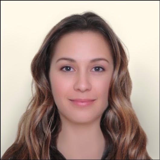
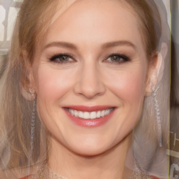
Most people would agree that the woman in Figure 1 is pretty. Can you guess her ethnicity ? Why is her skin flawless ? Well, she is not real. She is not completely virtual either. Her face is the average face of all female employees who worked at my company, Sight Commerce Inc., around 2011. It is difficult to pin point her ethnicity because, thanks to our excellent diversity record, she is part Caucasian, part Hispanic, part Asian and part Indian!
This history of face averaging is fascinating.
It all started with Francis Galton ( cousin of Charles Darwin ) who, back in 1878, came up with a new photographic technique for compositing faces by aligning the eyes. He thought that by averaging faces of criminals he could create the prototypical criminal face which in turn would help predict if someone is a criminal based on their facial features. His hypothesis turned out to be wrong; you cannot predict if a person is a criminal by looking at their photos.
However, he noted that the average face was always more attractive than the faces it was the average of.
Several researchers in the 1990s showed that people find facial averages much more attractive than individual faces. In one amusing experiment researchers averaged the faces of 22 miss Germany finalists of 2002. People rated the average face to be much more attractive than every one of the 22 contestants, including miss Berlin who won the competition. Ouch! Turns out Jessica Alba’s face is attractive precisely because her face is close to the average!
Shouldn’t an average be mediocre by definition ? Why do we find an average face attractive ? According to an evolutionary hypothesis called Koinophilia, sexually reproducing animals seek mates with average features because deviations from the average could indicate disadvantageous mutations. An average face is also symmetric because the variations in the left side and the right side of the face are averaged out.
How to create an average face using OpenCV ?
This post is part of a series that includes Facial Landmark Detection, Delaunay Triangulation, Face Morphing and Face Swap. We build on some of the concepts introduced in these previous posts. In fact Face Averaging is no different in theory from Face Morphing.
The steps for generating an average face given a set of facial images is described below. We make no assumptions about the size of the images or the size the faces in the images.
Step 1 : Facial Feature Detection
For each facial image we calculate 68 facial landmarks using dlib. Details about installing and using dlib can be found in my post on Facial Feature Detection. The figure on the left shows the 68 landmark points.
Step 2 : Coordinate Transformation
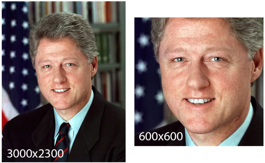
The input facial images can be of very different sizes. So we need a way to normalize the faces and bring them to the same reference frame. To achieve this we warp the faces to a 600×600 image such that the left corner of the left eye is at pixel location ( 180, 200 ) and the right corner of the right eye is at pixel location ( 420, 200 ). Let us call this coordinate system the output coordinate system and the coordinates of the original images the input coordinate systems.
How were the above points chosen ? I wanted to make sure the points were on a horizontal line, and the face was centered at about a third of the height from the top of the image. So I chose the corners of the eyes to be at ( 0.3 x width, height / 3 ) and ( 0.7 x width , height / 3 ).
We also know the location of the corners of the eyes in the original images; they are landmarks 36 and 45 respectively. We can therefore calculate a similarity transform ( rotation , translation and scale ) that transforms the points from the input coordinate systems to the output coordinate system.
![\[S=\begin{bmatrix}s_x \cos(\theta) & \sin(\theta) & t_x \\-\sin(\theta) & s_y \cos(\theta) & t_y\end{bmatrix}\]](https://learnopencv.com/wp-content/ql-cache/quicklatex.com-b6e614b5448854f2c83abcb6e5786774_l3.png)
![\[\begin{bmatrix}x_t \\y_t\end{bmatrix}=\begin{bmatrix}s_x \cos(\theta) & \sin(\theta) \\-\sin(\theta) & s_y \cos(\theta)\end{bmatrix}\begin{bmatrix}x \\y\end{bmatrix}+\begin{bmatrix}t_x \\t_y\end{bmatrix}\]](https://learnopencv.com/wp-content/ql-cache/quicklatex.com-46b93d3572bf6977c11de5e8d3da253d_l3.png)
To find the similarity transform that will transform the points from the input image coordinates to the output image coordinates we can use estimateRigidTransform
C++
// inPts and outPts are Vectors of points.
// The last parameter indicates we do not want a similarity
// transform and not a full affine transform.
cv::estimateRigidTransform(inPts, outPts, false);
Python
# inPts and outPts are numpy arrays of tuples
# The last parameter indicates we do not want a similarity
# transform and not a full affine transform.
cv2.estimateRigidTransform(inPts, outPts, False);
There is one little problem though. OpenCV requires you to supply at least 3 point pairs. This is silly because you can calculate a similarity transform using just two points. The good news is that we can simply hallucinate a third point such that it forms an equilateral triangle with the two known points and then use estimateRigidTransform as if we had three points pairs.
Once a similarity transform is calculated, it can be used to transform the input image and the landmarks to the output coordinates. The image is transformed using warpAffine and the points are transformed using transform.
Step 3 : Face Alignment
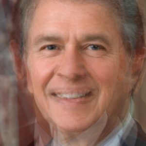
In the previous step we were able to transform all the images and the landmarks to the output image coordinates. All the images are now of the same size, and the two corners of the eyes are aligned. It may be tempting to obtain the average image by averaging pixel values of these aligned images. However if you did this, you will end up with an image shown on the left. Sure, the eyes are aligned, but other facial features are misaligned.
If you are a regular reader of this blog, you probably know the trick we are going to use next to bring the facial features in alignment.
If we knew which point in one input image corresponded to which point in another input image we could easily align the two images perfectly. However, we do not have that information. We only know the locations of 68 corresponding points in the input images. We will use these 68 points to divide the images into triangular regions. and align these regions before averaging pixel values.
You will benefit from reading my post on Face Morphing for more details on this alignment process. A less detailed description follows.
Calculate Mean Face Points
To calculate the average face where the features are aligned, we first need to calculate the average of all transformed landmarks in the output image coordinates. This is done by simply averaging the x and y values of the landmarks in the output image coordinates.
Calculate Delaunay Triangulation
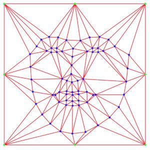
In the previous step we obtained the landmark locations for the average face in the output image coordinates. We can use these 68 points (shown in blue in Figure 6 ), and 8 points on the boundary of the output image (shown in green) to calculate a Delaunay Triangulation ( shown in red ). More details about Delaunay Triangulation can be found here.
Delaunay triangulation allows us to break the image into triangles. The result of Delaunay triangulation is a list of triangles represented by the indices of points in the 76 points ( 68 face points + 8 boundary points ) array. In the triangulation example shown below in the yellow box, we see than landmarks 62, 68 and 60 form a triangle, and 32, 50, and 49 form another triangle and so on.
[
62 68 60
32 50 49
15 16 72
9 8 58
53 35 36
… ]
Warp Triangles
In the previous step we calculated the average location of facial landmarks and used these locations to calculate a Delaunay triangulation to divide the image into triangles. In Figure 7, the left image shows Delaunay triangles on the transformed input image and the middle image shows the triangulation on the average landmarks. Note that triangle 1 in the left image corresponds to triangle 1 in the middle image. The three vertices of triangle 1 in the left image and the corresponding vertices in the middle image can be used to calculate an affine transform. This affine transform can be used to transform all pixels inside triangle 1 in the left image to triangle 1 in the middle image. This procedure when repeated for every triangle in the left image, results in the right image. The right image is simply the left image warped to the average face.
Step 4 : Face Averaging
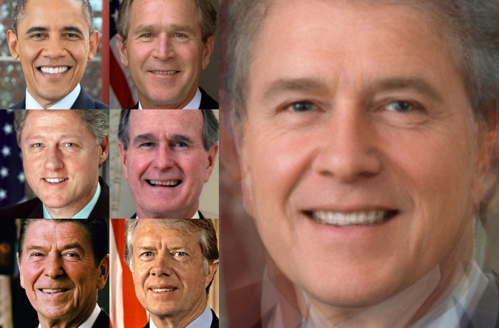
The previous step, when applied to all input images, gives us images that are correctly warped to the average image landmark coordinates. To calculate the average image, we can simply add the pixel intensities of all warped images and divide by the number of images. Figure 2 shows the result of this averaging. It looks much better than the average we obtained in Figure 5.
How do you think how the average President looks ? Would love to hear your response. To me, he looks fatherly and kind.
Face Averaging Results
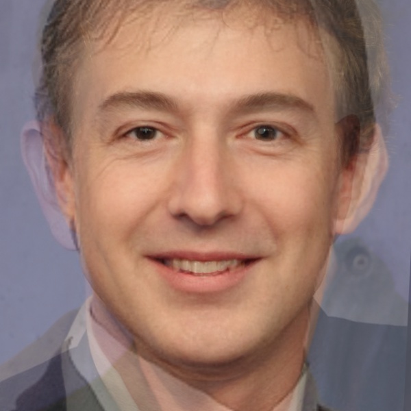
How does an average successful male tech entrepreneur look like ? Figure 8 below shows the average face of Mark Zuckerberg, Larry Page, Elon Musk and Jeff Bezos. I can’t find anything remarkable to say about this average entrepreneur except that he still has some hair left despite Jeff Bezos trying to hold the average down.
How does an average Oscar’s best actress winner look like ? Figure 9 below shows the average face of Brie Larson, Julianne Moore, Cate Blanchett and Jennifer Lawrence. The average good actress looks very charming! She also has better teeth than the average entrepreneur. No surprises here!
You can also make a symmetric face, by averaging a face and its mirror reflection. An example is shown below.

Image Credits
All the images of current and former presidents are in public domain and were downloaded from wikipedia.
I got permission to use the image in Figure 1. from Sight Commerce Inc.








100K+ Learners
Join Free OpenCV Bootcamp3 Hours of Learning