

DUSt3R (Dense and Unconstrained Stereo 3D Reconstruction) introduces a novel paradigm in multi-view 3D reconstruction, eliminating the need for predefined camera poses and intrinsics.
3D Reconstruction is one of the most fascinating yet challenging problems in computer vision. The applications of 3D Reconstruction are vast, ranging from interactive digital twins to robotic perception. Over the years, it has evolved from classical task specific geometric methods to modern deep learning based approaches. While deep learning shows great promise, most of the existing algorithms are extremely slow, computationally expensive making real time applications impractical.
If you have worked with NeRF or Gaussian Splatting, you know how time consuming and resource intensive it is to extract features and generate a dense 3D reconstruction, from a visual scene. Especially when dealing with unknown camera poses and missing intrinsics or images captured in the wild. But what if you could obtain a high quality initial point cloud map for your gaussian splats with fewer than 15 images and in just a few minutes all without requiring camera intrinsics?
That’s exactly what DUSt3R ( Dense and Unconstrained Stereo 3D Reconstruction) brings to the table. Developed by Naver Labs, it is a precursor to the almighty MASt3R, an advanced family of foundation models achieving the goal of “a unified 3D vision model” thereby capable of solving multiple downstream tasks and reducing complexity.
Key concepts discussed in this article are outlined as follows:
- Limitations of existing approaches.
- How DUSt3R presents a compelling alternative to SfM and MVS.
- Inference and Comparison results of DUSt3R v/s COLMAP Dense Reconstruction
If you’re someone just getting started with 3D computer vision, our series of articles will guide through the fundamentals of 3D Vision.
- 3D Reconstruction with Gaussian Splatting and NeRF
- Stereo and Monocular Depth Estimation
- Understanding Camera calibration and Geometry.
- Visual SLAM
- An overview of existing 3D Reconstruction methods
- Understanding DUSt3R, an Unified 3D Vision Model
- What is CroCo Pre-training Strategy?
- DUSt3R Training
- DUSt3R: Model Architecture
- DUSt3R Metrics
- Code Walkthrough of DUSt3R Inference Pipeline
- Understanding DUSt3R Scene Graph Strategies for Image Pairing
- Prediction and Global Alignment
- Comparison of DUSt3R v/s COLMAP MVS Results
- Testing DUSt3R on Hard Cases
- DUSt3R Limitations
- Key Takeaways
- Conclusion
An overview of existing 3D Reconstruction methods
Fundamentally, most 3D reconstruction system involves estimating correspondences between 2D pixels and a 3D point using triangulation. From a collection of 2D images captured at different camera viewpoints, classical Structure-from-Motion (SfM) / SLAM and Multi-View Stereo (MVS) methods aim to recover the 3D structure of the scene, taking camera intrinsics into account. However other methods also exists such as monocular depth estimators that can approximate the 3D scene using geometric priors.
The following image better illustrates different approaches involved in 3D reconstruction enabling multiple downstream tasks.

SfM and MVS
Traditional SfM and MVS pipeline, such as those implemented in widely used standard (defacto) tools like COLMAP involves multiple cascaded processing stages:
1. Sparse Reconstruction with SfM:

- Feature Extraction & Feature Matching: Descriptors or Keypoint Detection is performed using methods like SiFT or ORB followed by matching corresponding keypoints between two viewpoints. This is achieved by exhaustive search of image pairs to build a correspondence graph.
- Triangulation: The camera pose is initially estimated using two images, followed by triangulation to compute 3D points. From this, incrementally 3D points are refined by adding more view points to the scene.
- The camera poses and 3D points are optimized by Global Bundle Adjustment, which calculates cost values to minimize reprojection error between observed keypoint and their reprojected positions from the 3D model resulting in better convergence.
- To improve robustness, incorrect matches i.e. outliers are filtered using RANSAC.
While sparse reconstructions from SfM are a good starting point, they lack surface details. To address this, the COLMAP pipeline also includes Multi View Stereo Matching which can perform dense reconstruction on top of these sparse priors.
However in modern approaches, up to Bundle adjustment is typically done with COLMAP, while the MVS is often replaced with NeRF or Gaussian splatting as they offer more photo-realistic scene rendering.
2. Dense Reconstruction with MVS
For SfM in COLMAP, if EXIF metadata (focal length, principal point) is unavailable, pinhole camera intrinsics are estimated heuristically or set to default values. However, in MVS, camera intrinsics and extrinsics must be already known.

MVS, involves stereo matching techniques to calculate depth from disparity across different view points. From sparse maps obtained from SfM, more points are sampled along the epipolar line to produce dense point clouds. COLMAP MVS estimates depth using
- Geometric structures based on epipolar geometry
- Photometric depth based on pixel values.
Individual depth maps are later combined into a single 3D structure. Those that don’t respect epipolar geometry are filtered out. Geometric Ramification ensures that inconsistent matches are removed resulting in accurate correspondences (pixels observing the same 3D point).
Shortcomings of existing 3D reconstruction methods
- SfM and MVS, requires all camera parameters to be known to accurately produce dense point clouds.
- As we have understood, most methods rely on multiple view points, requiring a lot of images with sufficient viewpoint overlap, say around 60% for dense reconstruction. However, real world data is often sparse, has limited perspectives, and includes occluded objects making it hard to establish correspondences.
- Global Bundle adjustment is computationally expensive with a cubic complexity, making it difficult to scale.
- Monocular depth estimators offer straightforward approaches, but their depth predictions are approximations and project them into 3D with no camera intrinsics aren’t accurate. Additionally in this method, extracting features from textureless surfaces, and transparent or reflective surfaces is challenging leading to very less feature matches.
- Latest methods like 3D Gaussian Splatting and NeRF perform exceptionally well in 3D scene or novel view rendering, but they are scene specific (i.e. overfitted on a scene)s, requiring training per scene rather than generalizing to unseen environments.


Understanding DUSt3R, an Unified 3D Vision Model
As we see, the COLMAP pipeline involves a chain of complex sequential stages making them computationally intensive and time-consuming. With multiple moving components, these pipelines introduce potential noise and errors which can affect the reconstruction quality.
But what if we could skip or bypass all these intermediate steps? What if a model can produce an output that directly maps between 2D image pixel coordinates to 3D point correspondences?
This is exactly what DUSt3R achieves with its point map representation built upon a concept called Scene Coordinate regression (SCR) matching.
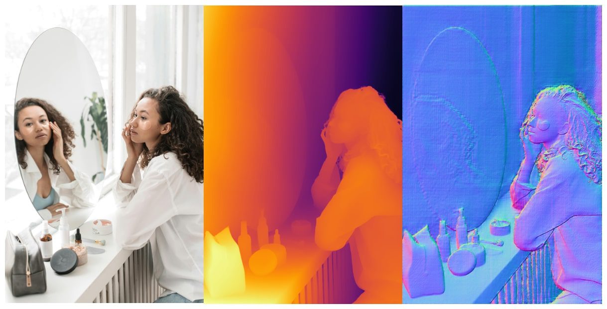
Pointmap Representation
A pointmap has the same dimensions as the input image, but instead of storing RGB values, encodes the x, y, z coordinates representing 3D point clouds. By training a network on point maps, the model learns:
- Geometric priors of the scene, enabling it to infer 3D structure.
- Direct 2D-3D correspondences, eliminating triangulation.
Pointmap representation encodes 3D scene geometry while preserving:
- 2D pixel consistency (Relative pose) across multiple views – preventing distortion.
- Direct 2D-to-3D space mapping – associating each pixel with a 3D point.
- Complete 3D scene geometry (Point Cloud) – maintaining spatial relationships.

Since the point map establishes a direct 2D-3D relation, all the scene parameters can be easily restored only from the point map including:
- Camera Intrinsics
- Depth Estimation
- Pixel Correspondences
- Camera Pose Estimation ([R | t] matrix)
- Dense 3D Reconstruction
Instead of processing into multiple independent stages, DUSt3R jointly learns the 2D patterns to 3D shapes in a single unified model. This eliminates the need for explicit triangulation which makes it inherently have excellent geometric and shape priors. As a result, DUSt3R reduces noise significantly. This makes DUSt3R, an end-to-end pipeline versatile and robust unified foundation model particularly for unknown camera poses in 3D Reconstruction tasks.
Both DUSt3R and MASt3R are built upon a common pretraining strategy called CroCo (Cross-View Completion), a primer research developed by the same team. CroCo serves as the core ingredient enabling these models as strong foundational architectures for geometric vision tasks. DUSt3R uses an asymmetric CroCo which is a slight variation of the original CroCo v1 framework. However before discussing Asymmetric CroCo, we will first review the original CroCo strategy, as it provides a better understanding of how the approach has evolved.
Before going into the nitty gritty of DUSt3R, let’s take a moment to see what DUSt3R is capable of:
What is CroCo Pretraining Strategy?
Let’s say given a pretext task of autocompletion from a single view, standard Masked Image Modelling (MIM), fills in missing pixels of masked content based on spatial information within the image. MIM works best for high level semantic tasks like classification and detection but it fails to capture the low level geometric structures of a scene.
This limitation arises because 3D reconstruction is inherently a multi-view problem. Training on just a single image isn’t sufficient as it lacks necessary geometric context and spatial consistency to infer any meaningful 3D representations. As a result it becomes challenging to transfer the MIM pretext task to low level downstream tasks like depth estimation, relative pose estimation and optical flow estimation.

So what’s the strategy?
Inspired from the design principles of MIM, CroCo framework introduces a second image from a different viewpoint as reference. This additional view guides the reconstruction process to perform a masked image model while conditioning on the second view. This approach is found to be very effective for low level downstream applications rather than high level semantics as it provides excellent spatial relationships and contextual cues between the masked view and reference view.
CroCo works better for 2D or 3D regression tasks even with larger mask ratios like 90%.

Mathematically CroCo can be formulated as,
(1) 
Diverse image pairs with sufficient overlap are chosen, and these images are divided into equal non overlapping patches. Similar to MIM, the first image is masked. Then, both the masked view and reference view are encoded into latent representation using a plain ViT encoder with shared weights.
The encoder processes the masked view ( ) also called query image and reference view
  independently in a siamese manner invariant to data augmentations, generating latent features. To enhance spatial understanding, the non-masked patch encodings from the first image attend to the reference image patch encodings via cross attention.
Finally, the objective of the CroCo ViT decoder (D_phi) is to predict those masked patches with Cross View Completion. It takes the masked view encoding conditioned on reference view encoding to reconstruct the target ( ) using an L2 Regression loss which predicts the missing pixel values.

Cross View Completion:
Let’s pay closer attention to the attention blocks of the decoder where cross view completion occurs. The latent encodings from the encoder are added with sinusoidal positional embeddings. As usual the positional embeddings help to retain the spatial context and indicate which patches in the flattened representations were masked.
These encodings pass through a series of transformer blocks consisting of Multi-Head Self attention and MLP Layers in the decoder. The authors experimented with two types of blocks,
- CrossBlock applies MHA on the first input non-masked tokens, followed by cross-attention with reference image tokens, balancing learnability and efficiency.
- CatBlock concatenates tokens from both images with additional learnable image embeddings and feeds to standard transformer decoder.
The decoder outputs 3 values (RGB) per pixel for each patch, resulting in a final representation of patch_size x patch_size x 3 (e.g. for a 16×16 patch, the output dimension is 16 x 16 x 3 = 768 values per patch).

Characteristics of a CroCo pretrained model:
- Has excellent geometric and scene understanding.
- Proven to learn important bricks of 3D vision
- Generic architecture easily adaptable to downstream task
- SOTA performance, outperforming task specific models
At the time of CroCo’s release, the authors achieved results by fine-tuning for each task separately with different checkpoints. However, it laid the foundation for a unified model approach. With DUSt3R, they successfully developed the model they had been aiming for, and the following year, they introduced MASt3R which is the next leap in their progression capable of predicting pixel correspondences and local features.
Pretraining Datasets of DUSt3R
DUSt3R is pretrained on a large corpus of data having equal proportion of synthetic and real data. While synthetic helps to get perfect geometric priors but real data adjusts the distribution for real world scenarios. This includes both indoor and outdoor scenes with 8.5M image pairs in total.
| Datasets | Type | N Pairs |
| Habitat | Indoor/ Synthetic | 100k |
| CO3Dv2 | Object-centric | 941k |
| ScanNet++ | Indoor / Real | 224k |
| ArkitScenes | Indoor / Real | 2040k |
| Static Thing 3D | Object / Synthetic | 337k |
| MegaDepth | Outdoor / Real | 1761k |
| BlendedMVS | Outdoor / Synthetic | 1062k |
| Waymo | Outdoor / Real | 1100k |
DUSt3R Training
Unlike CroCo, which follows a self-supervised strategy, DUSt3R is trained in a fully supervised manner with ground truth image pairs aligned in the same canonical reference frame. From each dataset, image pairs are randomly sampled to maintain equal data distribution.
The network is initially pretrained on 224×224 resolution images and then 512×512 for higher-quality reconstructions. To handle varying image ratios, images are cropped and resized ensuring the largest dimension remains 512.
Instead of starting from scratch, DUSt3R leverages an off-the-shelf CroCo pretrained model, utilizing its prior learned feature representations.
Loss Functions:
DUSt3R is trained using a scale invariant regression loss to prevent any ambiguity in scale differences between normalized ground truth and predicted point maps.
The training process is guided by two key loss functions:
1. 3D Regression Loss ( )
)
As we understood already, that regressing point map is a 3D regression problem, measuring a simple euclidean distance between predicted and ground truth point maps for valid pixels to maintain structural consistency.

where,
 represents the predicted 3D point for pixel i in view v.
 represents the ground truth 3D point.
 is the normalization factory, computed as the average distance of all valid points.
2. Confidence-Aware Loss ( )
)
In real world scenes, some pixels are harder to predict due to transparency, reflections or occlusions. To mitigate errors in these regions, the network also learns to output a confidence score for each pixel.
The final training objective is a confidence-weighted regression loss applied over all valid pixels.

Where,
 is the confidence score for pixel
  guarantees strictly positive confidence values i.e. greater than 1.
- Alpha is a hyper parameter for regularization, ensuring that the confidence doesn’t collapse to zero.
This helps model to assign lower confidence for uncertain areas, ensuring accurate 3D representation handling ill-defined points such as transparent, reflective or featureless surfaces (eg ; sky or glass):
Optimizations – Global Alignment
Unlike SfM, DUSt3R does not use Bundle Adjustment (BA) for minimizing 2D reprojection error. Instead it introduces first of its kind global alignment strategy, minimizing error in 3D space directly adjusting the camera pose and scene geometry.
When there are more than two images DUSt3R:
- Calculate pairwise relative pose estimation and build a pairwise connectivity graph finding the best possible matches by thresholding the pairs that have a bigger sum of confidence score.
- Optimises all pairwise pointmaps iteratively aligns them to a common reference frame. This is similar to BA, but faster and efficient converging quickly with few images.

where,
 → Global camera coordinate
 → Rigid transformation aligning point maps across views.
DUSt3R: Model Architecture

The architecture of DUSt3R looks similar to CroCo v1 with a slight modification with asymmetric design. The asymmetry comes from the use of two separate decoders rather than a shared decoder as seen in CroCo.

Patch Encodings
The encoder takes in a collection of RGB images and is patchified and rotary positional embeddings are added. Up until the encoder part, it is similar to CroCo where random patches are masked and the embeddings of first and second view are passed to the decoders. The encoder contains 24 x encoder blocks with self attention and MLP layers whose final embedding dimension is (1024, )
AsymmetricCroCo3DStereo(
 (patch_embed): PatchEmbedDust3R(
   (proj): Conv2d(3, 1024, kernel_size=(16, 16), stride=(16, 16))
   (norm): Identity()
 )
 (mask_generator): RandomMask()
 (rope): cuRoPE2D()
 (enc_blocks): ModuleList(
   (0-23): 24 x Block(
     (norm1): LayerNorm((1024,), eps=1e-06, elementwise_affine=True)
     (attn): Attention(. . . )


     (mlp): Mlp(
. . .
(fc2): Linear(in_features=4096, out_features=1024, bias=True)
)
   )
 )
CroCo v2 Stereo Decoder
DUSt3R introduces an additional decoder with the same layers for the second view tokens. and the features of first image and second image are cross attended. The decoder contains 12 x CrossBlocks with attention, cross attention and MLP layers with an output dimension of (768, ) per patch. Information is constantly shared between decoders for guiding the model to output properly aligned pointmaps.
(decoder_embed): Linear(in_features=1024, out_features=768, bias=True)

# DECODER 1
 (dec_blocks): ModuleList(
   (0-11): 12 x DecoderBlock(
     (norm1): LayerNorm((768,), eps=1e-06, elementwise_affine=True)
     (attn): Attention(. . .)
     (cross_attn): CrossAttention(. . .)
     (mlp): Mlp(
	. . .
(fc2): Linear(in_features=3072, out_features=768, bias=True)


)

# DECODER 2
 (dec_blocks2): ModuleList(
   (0-11): 12 x DecoderBlock(
     (norm1): LayerNorm((768,), eps=1e-06, elementwise_affine=True)
     (attn): Attention(. . .)
     (cross_attn): CrossAttention(. . .)
     (mlp): Mlp(
	. . .
	(fc2): Linear(in_features=3072, out_features=768, bias=True)


) ))
Decoder 1:
- Focuses on reconstructing the point map for the first image, generating 3D point clouds for that view.
- It predicts the red point map (X1,1, C1,1) which is expressed in terms of Camera 1. The Camera 1 is centered and posed along the z direction.
Decoder 2:
- Uses cross attention to align the point map of the second image relative to a common reference coordinate of the first image, effectively estimating the camera pose across views.
- It predicts the blue pointmap (X2,1, C2,1), where Camera 1 remains as a common reference frame. The positions and pose of Camera 2 are estimated relative to the Camera 1’s coordinate system, ensuring both point clouds are in the same coordinate system.
Downstream Head for DepthMap
Finally, two downstream DPT (Dense Prediction Transformer) regression heads are added. The out channels of the head is 4, where each head outputs the depth maps from which point maps(x, y, z coords of a 3D point cloud) and its associated confidence for each pixel are derived. The output pointmap is regressed up to an unknown scale. i.e. here, depth is relative not metric. The output pointmaps, while not accurate does closely correspond to physically plausible camera model.

## HEAD 1 - First view

(downstream_head1): PixelwiseTaskWithDPT(
   (dpt): DPTOutputAdapter_fix(. . .)
     (head): Sequential(
       (0): Conv2d(256, 128, kernel_size=(3, 3), stride=(1, 1), padding=(1, 1))
		. . .
       (4): Conv2d(128, 4, kernel_size=(1, 1), stride=(1, 1))
     )
     (act_postprocess): ModuleList( . . . )

# HEAD 2 - Second view
(downstream_head2): PixelwiseTaskWithDPT(
   (dpt): DPTOutputAdapter_fix(. . .)
     (head): Sequential(
       (0): Conv2d(256, 128, kernel_size=(3, 3), stride=(1, 1), padding=(1, 1))
		. . .
       (4): Conv2d(128, 4, kernel_size=(1, 1), stride=(1, 1))
     )
     (act_postprocess): ModuleList( . . . )
DUSt3R from a pair of images, predicts point maps from which camera parameters can be recovered. For monocular reconstruction, feed the input image twice, to obtain a point map where focal length can be estimated.

1. Point Matching or Pixel Correspondences


2. Visual Localization

3. Multi-view Pose Estimation
From the correspondences, DUSt3R employs algorithms like PnP (Perspective-n-Point) combined with RANSAC to robustly estimate the relative camera poses.

4. Monocular Depth Estimation (relative):
Relation between point map and depth map given camera intrinsics parameters,

X is expressed in its own camera coordinate(CC) frame. To convert it to another camera’s coordinate:

5. Multi-view Depth and 3D Reconstruction

6. Recovering Camera Intrinsics
 is represented in it’s own camera coordinate frame,

DUSt3R Metrics
DUSt3R is notably good at multi-view camera pose estimation and depth prediction tasks achieving SOTA performance without task-specific fine-tuning. It operates in zero-shot settings, generalizing across unseen query images. Across other tasks, it outperforms self-supervised baselines and delivers on par results comparable to supervised models.
However, while DUSt3R is extremely robust, it also falls short in accuracy compared to SOTA MVS baselines due to its regression based approach.

Until now, we have understood all the nitty gritty details about DUSt3R internal workings from a theoretical perspective. Now it’s time to take a closer look at the implementation details of DUSt3R pipeline.
For this, we will mostly adapt the inference code from original source `dust3r/dust3r/demo.py`, However we recommend, hitting the download code button and fill in your details to get access to all dataset files and point clouds outputs shown in the inference section.
Code walkthrough of DUSt3R Inference Pipeline
To run DUSt3R locally, simply clone the repository. DUSt3R utilizes modules from the CroCo repository, therefore make sure to install additional submodules recursively.
git clone --recursive https://github.com/naver/dust3r
cd dust3r
# if you have already cloned dust3r:
# git submodule update --init --recursive
!pip install -r requirements.txt
# Optional: you can also install additional packages to:
# - add support for HEIC images
# - add pyrender, used to render depthmap in some datasets preprocessing
# - add required packages for visloc.py
!pip install -r requirements_optional.txt
DUSt3R relies on RoPE positional embeddings for which you can compile some cuda kernels for faster runtime optionally.
cd croco/models/curope/
python setup.py build_ext --inplace
cd ../../../
For model checkpoints, we need to specify the model type directly as one of the arguments and `demo.py` will automatically download the model. Alternatively it can also be manually downloaded and placed under the checkpoints folder in the working directory.
mkdir -p checkpoints/
!wget https://download.europe.naverlabs.com/ComputerVision/DUSt3R/DUSt3R_ViTLarge_BaseDecoder_512_dpt.pth -P checkpoints/
There are three model variants based on input resolutions such as 224×224 or 512×512 and different head types including Linear and DPT.
| Modelname | Training resolutions | Head | Encoder | Decoder |
|---|---|---|---|---|
| DUst3R_ViTLarge_BaseDecoder_224_linear.pth | 224×224 | Linear | ViT-L | ViT-B |
| DUst3R_ViTLarge_BaseDecoder_512_linear.pth | 512×384, 512×336, 512×288, 512×256, 512×160 | Linear | ViT-L | ViT-B |
| DUst3R_ViTLarge_BaseDecoder_512_dpt.pth | 512×384, 512×336, 512×288, 512×256, 512×160 | DPT | ViT-L | ViT-B |
All the inference results shown throughout this article are inferred from the DUSt3R_ViTLarge_BaseDecoder_512_dpt checkpoint using a i7 13th gen, RTX 3080 Ti GPU with 12GB VRAM system. The memory requirements vary based on the number of input images and chosen global alignment method. We will discuss more about this in some time moving forward.
Import Dependencies
import argparse
import math
import builtins
import datetime
import gradio
import os
import torch
import numpy as np
import functools
import trimesh
import copy

from dust3r.utils.device import to_numpy
import matplotlib.pyplot as pl
The `demo.py` script provides a gradio interface for testing DUSt3R. It takes in the various arguments related to model resolution and other gradio-related configurations.
| Arguments | Description |
—model_name | Available models:- DUSt3R_ViTLarge_BaseDecoder_512_dpt (default)- DUSt3R_ViTLarge_BaseDecoder_512_linear- DUSt3R_ViTLarge_BaseDecoder_224_linear |
—weights | path to the model weights, eg:- checkpoints/DUSt3R_ViTLarge_BaseDecoder_512_dpt.pth |
—image_size | Supported resolutions by the models:- [512, 224] Default: resized to 512 |
—device | to use a different device “cpu” or “cuda” or “mps”, by default it’s “cuda” |
def get_args_parser():
   parser = argparse.ArgumentParser()
   parser_url = parser.add_mutually_exclusive_group()
   parser_url.add_argument("--local_network", action='store_true', default=False,
                           help="make app accessible on local network: address will be set to 0.0.0.0")
   parser_url.add_argument("--server_name", type=str, default=None, help="server url, default is 127.0.0.1")
   parser.add_argument("--image_size", type=int, default=512, choices=[512, 224], help="image size")
   parser.add_argument("--server_port", type=int, help=("will start gradio app on this port (if available). "
                                                        "If None, will search for an available port starting at 7860."),
                       default=None)
   parser_weights = parser.add_mutually_exclusive_group(required=True)
   parser_weights.add_argument("--weights", type=str, help="path to the model weights", default=None)
   parser_weights.add_argument("--model_name", type=str, help="name of the model weights",
                               choices=["DUSt3R_ViTLarge_BaseDecoder_512_dpt",
                                        "DUSt3R_ViTLarge_BaseDecoder_512_linear",
                                        "DUSt3R_ViTLarge_BaseDecoder_224_linear"])
   parser.add_argument("--device", type=str, default='cuda', help="pytorch device")
   parser.add_argument("--tmp_dir", type=str, default=None, help="value for tempfile.tempdir")
   parser.add_argument("--silent", action='store_true', default=False,
                       help="silence logs")
   return parser
To run the provided gradio demo run,
!python3 demo.py --model_name DUSt3R_ViTLarge_BaseDecoder_512_dpt

# Use --weights to load a checkpoint from a local file, eg --weights checkpoints/DUSt3R_ViTLarge_BaseDecoder_512_dpt.pth
# Use --image_size to select the correct resolution for the selected checkpoint. 512 (default) or 224
# Use --local_network to make it accessible on the local network, or --server_name to specify the url manually
# Use --server_port to change the port, by default it will search for an available port starting at 7860
# Use --device to use a different device, by default it's "cuda"
The inference gradio demo of DUSt3R will look as:
Dataset: Tanks&Temples/Family
To remove noise, we will apply mask_sky based on confidence values and adjust the confidence threshold accordingly.
If you have observed in the above demo, we chose one-ref as the scenegraph configuration, but what was it and why we chose that specifically?
Understanding DUSt3R Scene Graph Strategies for Image Pairing
The pipeline provides a structured way to prepare input image pairs (in image_pairs.py) for multi-view 3D reconstruction through image_pairs.py. It constructs a connectivity graph where:
- Edges represents current anchor image.
- Relations represent all matching images forming a pairwise graph.
The chosen scene graph strategy directly impacts global alignment convergence and computational efficiency. Each edge in the pairwise graph contributes to the overall reconstruction by linking shared visual content. This uses known camera poses, principal points and focal length optimizing the camera intrinsics and extrinsics iteratively.
The following are available scene graph strategies for pairing:
- Complete Pairing: (“complete”)
- Every image is paired with all previous images in the sequence.
For eg: Say you have images [A, B, C, D] in the sequence and the pairs generated will be: (B, A), (C, A), (C, B), (D, A), (D, B), (D, C). - It is computationally intensive, but can help the model in understanding the global context.
- Best suited for small datasets (let’s say < 15), where memory is constrained.
Note: From the community discussions, multiple users have reported with > 120 images, they find it hard to fit with complete pairing in a A100 (80GB VRAM) GPU.
- Sliding Window Pairing: (“swin”)
- Pairs each image with its adjacent images within a specified window size.
For eg: winsize = 2 for [A, B, C, D] image sequence, the pairs generated will be (A, B), (A, C), (B, C), (B, D), (C, D) - How is win_size determined?: The possible window size for each inference depends on the number of input images, it is half the size of total images provided by the user.
- Efficient for sequential frames (In our case, 360° video of a scene).
- Reduces computation by limiting pairwise comparisons to highly matching features in frames.
- Single Reference Pairing (“oneref”)
- Uses a fixed anchor image as reference viewpoint and pairs it with all other images. The reference id can be any idx from
0 to len(images) -1, chosen of our choice and is defaulted to 0.
For eg: (ref_id = 0) for [A, B, C, D] image sequence, the pairs generated are: (A, B), (A, C), (A, D) - Best for Large scale datasets, occupying less memory compared to “complete” and “swin” pairing.
The scene_graph_options utility in the interface helps to dynamically choose between these image pairing configurations.
from dust3r.image_pairs import make_pairs
def set_scenegraph_options(inputfiles, winsize, refid,scenegraph_type):
   num_files = len(inputfiles) if inputfiles is not None else 1
   max_winsize = max(1, math.ceil((num_files - 1) / 2))
   if scenegraph_type == "swin":
       winsize = gradio.Slider(label="Scene Graph: Window Size", value=max_winsize,
                               minimum=1, maximum=max_winsize, step=1, visible=True)
       refid = gradio.Slider(label="Scene Graph: Id", value=0, minimum=0,
                             maximum=num_files - 1, step=1, visible=False)
   elif scenegraph_type == "oneref":
       winsize = gradio.Slider(label="Scene Graph: Window Size", value=max_winsize,
                               minimum=1, maximum=max_winsize, step=1, visible=False)
       refid = gradio.Slider(label="Scene Graph: Id", value=0, minimum=0,
                             maximum=num_files - 1, step=1, visible=True)
   else:
       winsize = gradio.Slider(label="Scene Graph: Window Size", value=max_winsize,
                               minimum=1, maximum=max_winsize, step=1, visible=False)
       refid = gradio.Slider(label="Scene Graph: Id", value=0, minimum=0,
                             maximum=num_files - 1, step=1, visible=False)
   return winsize, refid
When the images are uploaded to the interface, the get_reconstructed_scene function will return the reconstructed scene. Initially RGB images are loaded into the memory. Now depending upon the chosen image pairing strategy, images will be paired and executes subsequent steps.
def get_reconstructed_scene(outdir, model, device, silent, image_size, filelist, schedule, niter, min_conf_thr,
                           as_pointcloud, mask_sky, clean_depth, transparent_cams, cam_size,
                           scenegraph_type, winsize, refid):
   """
   from a list of images, run dust3r inference, global aligner.
   then run get_3D_model_from_scene
   """
   from dust3r.utils.image import load_images, rgb
   imgs = load_images(filelist, size=image_size, verbose=not silent)

# # Duplicate the image for monocular reconstruction

   if len(imgs) == 1:
       imgs = [imgs[0], copy.deepcopy(imgs[0])]
       imgs[1]['idx'] = 1 # Assign an index to the duplicated image
   if scenegraph_type == "swin":
       scenegraph_type = scenegraph_type + "-" + str(winsize)
   elif scenegraph_type == "oneref":
       scenegraph_type = scenegraph_type + "-" + str(refid)

   pairs = make_pairs(imgs, scene_graph=scenegraph_type, prefilter=None, symmetrize=True)
Prediction and Global Alignment
The input images are passed to the inference(…) function where input images are processed as different views “view 1” & “view 2”.
1. Forward Pass to the AsymmetricCroCo3DStereo model (dust3r/model.py):
The model returns the final results as “pred 1” & “pred 2” where each prediction contains:
– Depth Map (depth) → Pixelwise depth values estimated by the model.
– 3D Point Map (pts3d) → (x, y, z) world coordinates of View 1 derived from depth using pseudo focal estimated by the model.
– Cross-View Correspondence (pts3d_in_other_view) → View 2’s 3D points transformed into View 1’s reference frame.
– Camera Pose (camera_pose) → Position and rotation matrix for 3D alignment.
This ensures direct 2D-to-3D mapping without the need for explicit triangulation.
2. Global alignment
After the CroCo model predicts the depth and point maps, the next step involves global alignment, which optimizes the model’s prediction for:
'Pw_poses' - Pairwise relative Pose,
'im_depthmaps' - Depth estimates for each image,
'im_poses' - camera positions and orientations in world frame, 'im_focals' - Pseudo focal length for each image.
Exporting 3D scene as GLB
Finally, the reconstructed 3D scene is saved as a .glb file and can be viewed in the interface as a mesh or dense point cloud. Point cloud visualization is smoother and less resource-intensive than mesh mesh rendering. To improve scene clarity, you can reduce the camera frustum size (“cam_size”) or disable it entirely by setting the slider to its min value (0.001). The main_demo(...) function brings everything together in a gradio-interface handling inference and scene visualization for DUSt3R pipeline.
The authors also have provided the training scripts and hyperparams used for DUSt3R. Training begins with a CroCo_V2_ViTLarge_BaseDecoder.pth at 224 resolution, followed by experiments at 512 resolution with checkpoints saved from previous steps. Check the repository main README for more details.
In the final section, we will compare DUST3R and COLMAP MVS outputs, where the results will speak for themselves – showing just how impactful DUSt3R is for dense reconstruction tasks.
From our experiments, on a 12GB VRAM system, when we feed more than 30 images, with “complete” scene pairing, we faced OOM error. In such scenarios switching to "one-ref" or "swin" to able to run within given compute demands. Interestingly, we didn’t observe a significant improvement in reconstruction quality across different strategies, though it needs further validation. If you have better insights or counterpoints, drop them in comments, we would be happy to learn from you.
Comparison of DUSt3R v/s COLMAP MVS Results
Our comparison is based on time and reconstruction fidelity assessed through a manual vibe check and interpretations of the predictions. The inference dataset used here include Meta CO3D , TanksAndTemples and our own captured scenes.
As mentioned earlier, inputs are resized to 512x384 or 384x512, where the maximum dimension (either height or width) is set to 512 while preserving the aspect ratio. For simplicity, in our visualization, size of the camera frustums are set to a minimal value.
Comparison 1:
The dataset is part of Meta CO3D_motorcycle dataset – motorcycle/427_59906_115672
DUSt3R (One-Reference Pairing, 204 Image Pairs):
- Took 1min 10 secs on a RTX 3080 Ti occupying 11.7GB VRAM.
- Uses one-ref strategy considering the memory constraints.

COLMAP MVS – Build with CUDA:
- Took 50+ minutes for dense multi-view stereo (MVS) reconstruction.
- Occupies less than 1GB VRAM during MVS stage.
With few images (around 10-16), COLMAP struggles to produce any meaningful results, as most feature matches gets filtered out. For the above motorcycles subset, we selected 16 unique views with minimal overlap and processed them with COLMAP. Only two viewpoints made it to the dense reconstruction stage, and there weren’t enough correspondences, resulting in sparse blobs of point clouds. However with DUSt3R as expected, it generated high quality point maps.
Comparison 2:
We captured this dataset by placing a DSLR camera stationary on a table and moving around it to capture all possible view of the scene. To access this dataset, check out the Project link that is shared once you download the code.
DUSt3R: Took 51 secs for 102 images with 204 image pairs with one-ref strategy.

COLMAP : Took more than 50 minutes for 102 images
Comparison 3:
The dataset is subset of Meta CO3D_teddybear dataset – teddybear/34_1479_4753
DUSt3R: Took 38 secs for 56 images with one-ref strategy.

COLMAP: With the same 56 images subset, the results didn’t match the quality of the one shown below. So we, processed the entire 202 images files from the original dataset collection to achieve better dense reconstruction and it also took around 1 hour.
In every case, DUSt3R outperformed COLMAP in both reconstruction quality and processing time, making it the clear winner for in our dense reconstruction comparison. However, we haven’t tested it against other dense reconstruction approaches yet.
Testing DUSt3R on Hard Cases
To push DUSt3R to its limits and evaluate its ability to “grok” complex scenes, the authors tested it under challenging conditions. They have also discussed a few scenarios where the results were surprisingly good, and we’ll discuss some of them here.
Case 1: Opposite view Matching
Two opposite view of a subject are given, and the reconstruction is pretty much intact structurally without deformation or holes. This demonstrates DUSt3R’s exceptional understanding of the scene even with sparse view points.
Case 2: Impossible Matching – Without Overlap
From the results below, we can observe reconstruction gaps at the light reflections next to the blue ring, In this case, for OpenCV University office entrance scene, we captured two images that has almost no overlap in the camera poses similar to the example discussed in the paper. If we had another image of the same point in the scene with some overlap to red camera pose, DUSt3R could refined its point map prediction using the additional view for better reconstruction.
Yet with just two images with no overlap, the result is quite realistic and impressive isn’t it?
Case 3: Larger Scenes Reconstruction
Finally, we tested DUSt3R on the TanksAndTemples – Church , to check how well it holds up for large-scale scenes. The prediction preserved intricate architectural and geometric details. DUSt3R maintains strong fidelity with minimal distortions. For this, we carefully curated only the first 0- 50 frames that were unique.
DUSt3R Limitations
- DUSt3R is robust but it lacks accuracy because it’s based on regression. In the MVS benchmark on DTU the overall distance (Cher distance in mm), is 1.741 mm without any camera parameters (GT), which is far from SOTA (0.295 mm less is better).
- For those looking for scaling terms, DUSt3R is scale-invariant, meaning there is no guarantee on the scale. With MASt3R, we can get metric monocular depth, metric binocular point map predictions.
- DUSt3R is built for dense reconstruction, and not for novel view synthesis, therefore it can’t fill in those missing gaps like NeRFs.
- Unlike Gaussian splats, which work well on reflective surface, DUSt3R faces challenges in reconstructing surfaces that have harsh lighting variations in certain instances.
- Not all accurate reconsruction leads to accurate visual localization as DUSt3R isn’t trained explicitly for matching, affecting its localization accuracy. This is the key improvement that MASt3R brings in.
- When there are too much overlapping camera poses, we see that reconstruction structure from DUSt3R gets collapsed rendering poor results.
- When the number of images are more, say > 120, DUSt3R inference, even with one-ref image pairing, requires more more than 16GB of VRAM.
Individuals and enterprises looking to integrate DUSt3R in your workflow and projects, should note that it is licensed under non-commercial (CC BY-NC-SA 4.0).
Key Takeaways
- DUSt3R introduces a new paradigm in 3D Reconstruction with a unified model capable of solving downstream tasks. While DUSt3R’s reconstruction mesh looks quite realistic, it still lacks the photo-realism that Gaussian Splat can offer. To address this, the community introduced InstantSplat which integrates MASt3R, delivering impressive results at high speed.
💡 In hindsight, while capturing custom scenes, it is recommended to move the camera around the subject rather than keeping it fixed and rotating the scene. Keeping the background static results in poor reconstruction, likely because the model struggles to extract diverse features. Additionally, minimal camera pose variation would have negatively impacted results.
Conclusion
We explored DUSt3R’s model architecture and training strategy in detail, comparing it against the Multi View Stereo Dense reconstruction using COLMAP. DUSt3R is a remarkable research addressing the practical challenges associated with existing methods from Naver Labs. Kudos to the team!
Be sure to check out our other articles and subscribe to our weekly updates to stay informed about our upcoming articles in this series.
References
- DUSt3R: Geometric 3D Vision Made Easy
- MV-DUSt3R+: Single-Stage Scene Reconstruction
- CroCo: Self-Supervised Pre-training for 3D Vision Tasks
- 3D Computer Vision Reading Group Session
- From CroCo to MASt3R: A Paradigm Change in 3D Vision Talk