Introduction to LiDAR SLAM: LOAM & LeGO-LOAM - Paper & Code Explained with ROS 2

LiDAR SLAM is a crucial component in robotics perception, widely used in both industry and academia for its efficiency and robustness in localization and mapping. In robotics perception research, LiDAR SLAM stands as a distinct field due to the variety of scenarios it must handle, such as indoor and outdoor environments, high speed of the ego-vehicle, dynamic objects, varying weather conditions, and the need for real-time processing etc. These complexities make LiDAR SLAM a critical area of study and innovation.

It’s fascinating how LiDAR SLAM can produce such structured and dense maps. At first glance, these maps might seem like the output of a deep learning model, but they are the result of sophisticated mathematical techniques and computer science principles. The field of LiDAR SLAM has evolved significantly, with research expanding each year from traditional mathematical approaches to incorporating deep learning methods, making it a rich and dynamic area of study.

This is the fifth article in our robotics series. So far, we’ve explored Monocular SLAM using OpenCV Python, provided a setup guide for ROS 2 with Carla, and dedicated an article to the workings and internals of ROS 2. In this post, we’ll understand LiDAR SLAM, focusing on two groundbreaking papers on LiDAR Odometry and Mapping:

LOAM: Lidar Odometry and Mapping in Real-time
LeGO-LOAM: Lightweight and Ground-Optimized Lidar Odometry and Mapping on Variable Terrain

We have provide a detailed mathematical understanding of both papers and a code explanation for LeGO-LOAM. Finally, we’ll show you how to run LeGO-LOAM in ROS 2. A thorough understanding of LiDAR SLAM is crucial, as we will utilize it in our final project of this blog post series: Building a 6DoF Autonomous Vehicle for Static Obstacle Avoidance Using ROS 2 and Carla.

NB: To set up ROS 2, refer to our ROS 2 Carla setup article, as we’ll be using it in this post.

Download Code To easily follow along this tutorial, please download code by clicking on the button below. It's FREE!

Click here to download the source code to this post

What is LiDAR SLAM?

The problem statement of LiDAR SLAM is formulated as follows,

Input: Given, a sequence of LiDAR scans of the environment from time $t = 0$ , to $t = n$ , represented as, $I = { I_0, I_1, I_2, ..., I_n}$ .

Output: Find the trajectory of the LiDAR (robot) $X = {x_1,x_2,x_3,...,x_n}$ , $x_{n}$ is the pose ( $x, y, z, roll, pitch, yaw$ ) of the LiDAR and the map of the environment $M = {p_1,p_2,p_3,...,p_n}$ , $p_n$ represents the 3D coordinates of the point cloud points corresponding to the environment. In the below image we represented the position of the LiDAR w.r.t the World coordinate as $T^{W}_L$ .

LiDAR SLAM Problem Statement

LiDAR Odometry and Mapping (LOAM) — Figure 1: LiDAR SLAM Problem Statement

Algorithm:

LOAM is similar to Visual SLAM. There are always these common steps,

Extract feature points (corner and planar points) from the LiDAR scan at time $t=0$ .
Establish correspondences for these feature points between the scan at time $t=0$ and the subsequent scan at time $t=1$ .
Estimate the LiDAR’s ego-motion (its movement and orientation) by minimizing the distance between corresponding feature points.
Align the current scan with the previous scan using the estimated ego-motion to produce a coherent point cloud map.
Apply backend optimization algorithms to refine the LiDAR’s pose and construct an accurate, consistent map of the environment.

Types of Approach to LiDAR SLAM

LiDAR SLAM stands out from visual SLAM with its high mapping accuracy, stability, and resistance to issues like illumination changes and scale drift, making it ideal for large-scale applications. The integration of multi-sensor fusion, such as LiDAR-Inertial, LiDAR-Visual, and LiDAR-Inertial-Visual systems, further enhances localization accuracy and robustness, addressing challenges like motion distortions, occlusions, and long-term mapping. This advancement in LiDAR SLAM technology is driving significant progress in intelligent perception applications such as autonomous driving, military navigation, and deep underground space/terrain exploration.

Main Street Autonomy Lidar mapping and odometry demo

LOAM paper C++ — Figure 2: Demo of LiDAR SLAM by Main Street Autonomy

Based on the literature survey, we can understand that research has mostly focused on 4 types of LiDAR-only Odometry/SLAM methods.

Feature Based: Extracts distinct geometric features such as edges and corners from lidar data to align and match points.
Direct Methods: Directly minimizing the difference between Lidar scans to calculate the orientation and translation of Lidar. Direct methods are much easier to implement from an implementation point of view.
Projection Based: Projects LiDAR data onto 2D planes or images for easier integration and processing with other sensor data.
Deep Learning Based: Employs deep neural networks to automatically learn and extract features from LiDAR data for localization and mapping eg: LO-Net, L3-Net, LiDAR-MOS etc.

Types of LiDAR SLAM Methods

LiDAR Odometry and Mapping (LOAM) — Figure 3: Types of LiDAR SLAM Methods

In this article, we will focus mainly on the featured-based LiDAR SLAM solution, specifically the LOAM literature, covering Zhang & Singh et al. paper on LiDAR SLAM and also LeGO-LOAM.

Paper Summary : LOAM – LiDAR Odometry and Mapping in Real-time

LOAM (LiDAR Odometry and Mapping) is the most classic and widely used method for LiDAR SLAM. A lot of work on feature based LiDAR SLAM has been inspired by this work such as LeGO-LOAM, V-LOAM, F-LOAM etc. The LOAM algorithm is as follows,

LOAM System Design

Above is the system design of LOAM (LiDAR Odometry and Mapping).

LiDAR scan points $\bm{\hat{P}}$ are collected and sent to Point Cloud Registration. The points are w.r.t the LiDAR Coordinate System.
Point Cloud Registration combines all the points during a sweep (360 rotation of the scan). The final output scan is represented as $\mathbf{P}_k$ .
The LiDAR odometry module estimates the motion of the LiDAR sensor over time by analyzing the registered point cloud $\mathbf{P}_k$ . The Odometry module uses the LiDAR motion transforms to undistort the point cloud $\mathbf{P}_k$ .
The LiDAR Mapping module takes the Undistorted point cloud $\mathbf{P}_k$ and computes the transformation that best aligns the current point cloud with the global map. This helps to refine the other input coming from lidar odometry.
Finally, the pose transforms published by the two algorithms are integrated to generate a transform output that maintains a continuous and smooth estimate of the LiDAR’s pose at a rate of around 10 Hz.

The process of how LiDAR SLAM works is similar to Visual SLAM. We will go through these points one by one. Loop closure is an important part of SLAM. The problem it solves is that, when the ego vehicle arrives at the area that it has already visited before it should be able to recognize the place and adjust its pose and map accordingly. LOAM doesn’t have any loop closing, you can see that from the below video,

LOAM Loop closure

Explain LOAM paper code in C++

Feature Point Extraction

Feature points are defined as edge points and planar points. But, how to decide if any point is an edge or planar? For that the authors defined a term $c$ to evaluate the smoothness of the local surface,

$\Large c$ = $\dfrac{1}{|S| \cdot |\mathbf{X}^L_{(k,i)}|}$ $\|\sum_{j \in S, j \neq i} ( \mathbf{X}^L_{(k,i)} - \mathbf{X}^L_{(k,j)} )\|$

Let, $S$ be the set of consecutive points around $i$ , captured by the laser scanner. if $P_k$ is a LiDAR point cloud data from sweep $k$ , and $(i,j,k,...,n)$ are the series of points captured by the LiDAR during scan $k$ , then $S$ would be a subset of these points, including $i$ and its immediate neighbours.
∥ $X_{(k,i)}^L$ ∥ denotes the norm of the vector $X_{(k,i)}^L$ (coordinates of point $i$ , $i \in P_k$ , in $L_k$ ).
$\left\|\sum_{j \in \mathcal{S}, j \neq i}\left(\boldsymbol{X}_{(k, i)}^L-\boldsymbol{X}_{(k, j)}^L\right)\right\|$ represents the sum of the differences between the point $X_{(k,i)}^L$ and each point in $X_{(k,j)}^L$ in set $S$ , excluding the point $i$ .

How does the above equation represent a surface smoothness?

A lower value of $c$ indicates that the neighbouring points are close to point $i$ , implying a smoother local planar surface. On a planar surface patch, the neighbouring points around a point $i$ will be closely aligned and evenly spaced.
A higher value of $c$ suggests greater deviation among the neighbouring points, indicating a rougher or more irregular local surface. This indicates an edge point. For a point identified as an edge, there should be a significant change in the surface’s orientation or a sharp discontinuity.

To evenly distribute the feature points within the environment, we separate a scan into four identical sub-regions. Each sub-region can provide maximally 2 edge points and 4 planar points. A point $i$ can be selected as an edge or a planar point only if its $c$ value is larger or smaller than a threshold, and the number of selected points does not exceed the maximum.
— LOAM: Lidar Odometry and Mapping in Real-time

By ensuring an even distribution of feature points in the four sub-regions, the overall quality, accuracy, and robustness of the scan analysis and subsequent applications (like mapping, object recognition, and navigation) are significantly improved.

How to select feature points?

Feature points are chosen based on their smoothness values: the sharpest edges (highest $c$ values) and the flattest surfaces (lowest $c$ values). When selecting these points:

There’s a limit on how many can be chosen in each area.
Points that are too close to already selected ones are skipped.
Points on surfaces parallel to the laser beam or near edges of hidden areas are also avoided.

LOAM Feature Extraction

Robotics Perception — Figure 5: LOAM Feature Selection

The above diagram represents the third point visually. Figure 5 (a), shows that point B is in a surface patch parallel to the laser beam, but point A’s surface has an angle with the beam, so point A is taken as a feature point.

In Figure 5 (b), point A is not taken as a feature point because even though from the current point of view, it seems occluded, but from a different perspective, it might be observable, which makes it unreliable.

Feature Correspondences

LOAM Scan Re-projection

lidar odometry and mapping ros — Figure 6: LOAM Scan Re-projection

Say, $t_k$ is the starting time of a sweep k, the point cloud received during the sweep is $P_k$ . Now the 2nd sweep $k+1$ happens, the starting time can be thought as $t_{k+1}$ , and the points collected during the sweep is $P_{k+1}$ . To have all the scanned points in the same time stamp we reproject the $P_k$ points at $t_{k+1}$ , these re-projected points represented as $\overline{P}_k$ .

Now, that we have both the point clouds in the same timestamp we can find the correspondences. We take the $P_{k+1}$ and find a set of edge points $\mathbf{E}_{k+1}$ and planar points $\mathbf{H}_{k+1}$ from the LiDAR point cloud using the methodology discussed in the previous step. Then we find edge points from $\bar{P}_k$ as the correspondences for the points in $\mathbf{E}_{k+1}$ , and planar patches as the correspondences for the points in $\mathbf{H}_{k+1}$ . At each iteration, $\mathbf{E}_{k+1}$ and $\mathbf{H}_{k+1}$ are reprojected to the beginning of the sweep using the currently estimated transform, say after reprojection it’s named as $\mathbf{\hat{E}}_{k+1}$ and $\mathbf{\hat{H}}_{k+1}$ .

LOAM Feature Correspondences

LiDAR Odometry — Figure 7: LOAM Feature Correspondences

At $t = \tau -1$ we have point cloud $P_k$
At $t = \tau$ , we get $\mathbf{H}_{k+1}$ and $\mathbf{E}_{k+1}$ and re-project $P_k$ to get $\bar{P}_k$ . The orange line represent that scan line.
At $t = \tau + 1$ , we reproject $\mathbf{H}_{k+1}$ and $\mathbf{E}_{k+1}$ to get $\mathbf{\bar{E}}_{k+1}$ and $\mathbf{\bar{H}}_{k+1}$ .
There are also two consecutive scans after $t = \tau$ , represented with two blue lines.

Now the task is to find the feature correspondences, between a point from E_bar with point in those two consecutive scans and the re-projected scan. Given, $i$ , a point from $\mathbf{\bar{E}}_{k+1}$ , $j$ (a point found from $\bar{P}_k$ ) and $l$ (a point found from one of those consecutive scans) are the two points that are closest neighbour of $i$ . Finally, $(j, l)$ forms the edge line correspondence of $i$ . The edge line is represented by two points.

A planar patch is represented by three points. Say $i$ is a point where $i \in \mathbf{\bar{H}}_{k+1}$ . As a correspondence of i we need to find 3 points. Similar to the last paragraph, we find the closest neighbour of $i$ in $\bar{P}_k$ , denoted as $j$ . Another point $l$ found from the same scan as $j$ given its closest to $i$ , and another point $m$ is found from one of the two consecutive scans. This guarantees that the three points are non-colinear.

We compute the distance between the feature points to its correspondences and minimize them to compute the LiDAR motion. We compute the distance between the feature edge point and the correspondence edge line using equation $(1)$ , and the distance between the feature planar point to its correspondence planar patch using equation $(2)$ .

feature edge and planner patch distance equations LOAM

How to run LOAM on ROS 2

Where, $\bar{X}_{(k+1,i)}$ , $\bar{X}_{(k,j)}$ , and $\bar{X}_{(k,l)}$ are the coordinates of points $i$ , $j$ , and $l$ in $L$ ( $L$ means LiDAR frame of reference), respectively and $\bar{X}_{(k,m)}$ is the coordinates of point $m$ in $L$ .

Estimate the LiDAR Motion

Now that we have calculated correspondences we can use that to calculate the LiDAR ego-motion. LiDAR motion has 6-DoF. We can linearly interpolate the pose transform within a sweep for the points that are received at different times.

Let $t$ be the current timestamp, and recall that $t_{(k+1)}$ is the starting time of sweep $k+1$ . From time $t_{k+1}$ to $t$ the lidar motion can be defined as $T^L_{k+1}$ . Say, at time $t_i$ we get some point. So the transform, $T^L_{(k+1,i)}$ (represented as ( $x, y, z, roll, pitch, yaw$ )) from time $t_{k+1}$ to $t_i$ , can be calculated using,

Lidar pose interpolation LOAM

Difference between Visual SLAM and LiDAR SLAM

Apart from reducing the distance between the feature point and correspondences, we also need to establish a geometric relationship between $\mathbf{H}_{k+1}$ and $\mathbf{\bar{H}}_{k+1}$ or $\mathbf{E}_{k+1}$ and $\mathbf{\bar{E}}_{k+1}$ . Below equation represents that,

3D to 3D transformation LOAM
LOAM: LiDAR Odometry and Mapping in Real-time

Here,

$\mathbf{X}^L_{(k+1,i)}$ : The coordinates of a point $i$ in $\mathbf{E}_{k+1}$ (set of edge points) or $\mathbf{H}_{k+1}$ (set of planar points).
$\mathbf{\bar{X}}^L_{(k+1,i)}$ : The corresponding reprojected point in $\mathbf{\bar{E}}_{k+1}$ (reprojected edge points) or $\mathbf{\bar{H}}_{k+1}$ (reprojected planar points).
$\mathbf{T}^L_{(k+1,i)}(a : b)$ : The a-th to b-th entries of the LiDAR pose $\mathbf{T}^L_{(k+1,i)}$ , representing translation or displacement.
$R$ : A rotation matrix defined by the Rodrigues formula.

Observed correctly, you can understand that it’s the 1st equation of the Epipolar Geometry section from the monocular slam blog post, explaining the 3D to 3D transformation from $\mathbf{\bar{X}}^L_{(k+1,i)}$ to $\mathbf{X}^L_{(k+1,i)}$ .

Rodrigues Formula

The Rodrigues formula is a mathematical expression used to convert a rotation vector (axis-angle representation) into a rotation matrix.

Given a rotation vector $\mathbf{\alpha} = [\alpha_x, \alpha_y, \alpha_z]^T$ , the magnitude $\theta = \|\mathbf{\alpha}\|$ represents the angle of rotation, and the unit vector $\mathbf{u} = \frac{\mathbf{\alpha}}{\theta}$ represents the axis of rotation. The rotation matrix $R$ can be computed using the Rodrigues formula:

$\theta$ is calculated as,

and $\omega$ is calculated as,

$\hat{\omega}$ is the skew symmetric matrix of $\omega$ .

LiDAR Transformation Calculation

Now that we have the distance equations $(1) & (2)$ and the projection point relation $(a)$ , using those authors came up with more simpler version of distance equations, where we can minimize the distance to recover the transformation $T$ (LiDAR motion from time $t_{k+1}$ till $t$ ). The geometric relationship between an edge point in $E_{k+1}$ and the corresponding edge line (found from feature correspondences) and points in $H_{k+1}$ and corresponding planar patches (found from feature correspondences) is derived as,

feature distance calculation function

Explain LOAM paper code in C++

Authors combine these two equations to obtain a nonlinear function,

transformation calculation function

What is LiDAR Odometry and Mapping

This nonlinear function is solved by minimizing $d$ towards zero. To do that first this nonlinear function can be linearized and represented as a least squares problem. This involves minimizing the sum of squared residuals:

The residual function $f(\mathbf{T}_L^{k+1})$ can be approximated linearly around the current estimate $\mathbf{T}_L^{k+1}$ using the Jacobian matrix:

state estimation from Jacobian matrix

visual lidar odometry and mapping low drift robust and fast

Here,

$\Delta \mathbf{T}$ represents a small change in the parameters.
$\mathbf{J}$ is the Jacobian matrix of $f$ with respect to $\mathbf{T}_L^{k+1}$ .
$\mathbf{T}_L^{k+1}$ is the current estimate of the transformation.

In a least squares problem, we aim to minimize the sum of squared residuals:

lidar transformation estimation optimization objective

LiDAR Odometry

Using the linear approximation, this can be written as:

linear approximation

LiDAR Odometry and Mapping (LOAM)

Expanding this, we get:

Simplifying, this becomes:

lidar transformation equation

How to run LOAM on ROS 2

To minimize this quadratic form, we take the derivative with respect to $\Delta \mathbf{T}$ and set it to zero:

pose estimation optimization objective

lidar odometry and mapping ros

The derivative is:

LOAM: LiDAR Odometry and Mapping in Real-time

LiDAR Odometry

Rearranging, we get the normal equation:

To solve for $\Delta \mathbf{T}$ :

From the Levenberg-Marquardt algorithm, a damping factor $\lambda$ is introduced to combine the gradient descent and Gauss-Newton methods, improving the convergence properties. The update equation becomes:

$\Delta \mathbf{T} = -(\mathbf{J}^T \mathbf{J} + \lambda \operatorname{diag}(\mathbf{J}^T \mathbf{J}))^{-1} \mathbf{J}^T \mathbf{d} \quad \quad \, \dots \, \text{(c)}$

Finally, the parameters are updated using the computed $\Delta \mathbf{T}$ :

LiDAR Odometry Pseudo Code

Now that we have derived the motion estimation equation, it would be very easy to iterate through the LiDAR Odometry Algorithm. If you were not able to follow in the previous steps, its your time to catch up. We will be referencing the line numbers mentioned in the below image to explain each step.

LOAM Odometry Pseudo code

LOAM paper C++

Run LOAM on ROS 2

Robotics Perception — Figure 8: LOAM Odometry Pseudo code

Inputs are,

$\overline{P}_k$ = Reprojected pointcloud captured in the k-th sweep
$P_{k+1}$ = The point cloud from k+1-th sweep
$\mathbf{T}_{k+1}^{L}$ = lidar pose transform between time $[t_{k+1}, t]$

Outputs are,

$\overline{P}_{k+1}$ = Reprojected $P_{k+1}$ to $t_{k+2}$ and form $\overline{P}_{k+1}$
$\mathbf{T}_{k+1}^{L}$ = updated $\mathbf{T}_{k+1}^{L}$

Say, there is a car with LiDAR attached to it. to get the LiDAR odometry we follow the above algorithm,

at $t=0$ (LiDAR starts capturing scans), we get a $P_k$ .

at $t=1$ we get $P_k+1$ .

Say the transformation from $t=0$ to $t=k+1$ is $\mathbf{T}_{k+1}^{L}$ . At the beginning $\mathbf{T}_{k+1}^{L}$ set to 0 (line 4-5), because we consider the starting point as the coordinate center.

In line 7, feature points from $\mathbf{H}_{k+1}$ and $\mathbf{E}_{k+1}$ are captured and stored based on the $c$ values. For a $N$ number of iteration we, find the edge line correspondences, and compute the edge feature point to edge line distance using the equation $(3)$ and the resulting equation is stacked in the form of equation $(b)$ (line 9-11). Again for the planar feature points we do the same as above (line 12-14).

Compute the bisquare weights for each row of the finally formed $(b)$ equation. Here, bisquare weight is a weight assigned to each data point based on its residual (d), reducing the influence of points with large residuals (outliers) [Line 15].

In line 16 we update the $\mathbf{T}_{k+1}^{L}$ based on the equation $(c)$ . If the distance comes to a minimum (optimization converges), we break the loop.

At the end of the $P_{k+1}$ sweep, $P_{k+1}$ is reprojected to $t_{k+2}$ to form $\overline{P}_{k+1}$ and we return, estimated $\mathbf{T}_{k+1}^{L}$ and $\overline{P}_{k+1}$ . This $\mathbf{T}_{k+1}^{L}$ , $\overline{P}_{k+1}$ and the scan at $t_{k+2}$ will be used as an input in the next iteration. Else, we directly return the updated $\mathbf{T}_{k+1}^{L}$ [Line 21-27].

LiDAR Mapping

Mapping part is the easiest part of LOAM. As we are considering the vehicle starting position as the world coordinate center, the LiDAR pose transform, w.r.t LiDAR and World is same $(\mathbf{T}_{k}^{L} = \mathbf{T}_{k}^{W})$ .

The output of LiDAR Odometry is $\mathbf{T}_{k}^{L}$ and the undistorted point cloud in LiDAR coordinate.

The problem is, to bring the point cloud in the world coordinate and add the transform of LiDAR pose to stitch the scans. Here the 3D to 3D transformation equation will come to play,

$X^W = X^L R + t = X^L * T^W$

LOAM Mapping

What is LiDAR Odometry and Mapping

Explain LOAM paper code in C++

How to run LOAM on ROS 2

Difference between Visual SLAM and LiDAR SLAM — Figure 9: LOAM Mapping

The above image explains the process in detail,

The blue curve represents the LiDAR pose on the map $\mathbf{T}_k^W$ generated by the mapping algorithm at sweep $k$ .
The orange curve shows the LiDAR motion during sweep $k+1$ , $\mathbf{T}^W_{k+1}$ computed by the odometry algorithm.
Using $\mathbf{T}^W_k$ and $\mathbf{T}^L_{k+1}$ , the odometry algorithm projects the undistorted point cloud onto the map as $\tilde{\mathbf{Q}}_{k+1}$ (green line segments), matching it with the existing map cloud $\mathbf{Q}_k$ (black line segments).
Based on this $\tilde{\mathbf{Q}}_{k+1}$ and $\tilde{\mathbf{Q}}_{k}$ matching, lidar pose $\mathbf{T}^W_{k+1}$ is being optimized.

LeGO-LOAM Paper Summary

LeGO LOAM paper is an extraction of the LOAM paper. The novelty of this LiDAR SLAM method lies in incorporating ground segmentation to enhance feature extraction and two step pose optimization. The overall system is divided into five modules,

LeGO-LOAM System Design

LiDAR Odometry and Mapping (LOAM)

LOAM: LiDAR Odometry and Mapping in Real-time

LiDAR Odometry — Figure 10: LeGO-LOAM System Design

Ground Segmentation

Ground segmentation is done by projecting the 3D points in a 2D plane. This projection creates a range image also known as a depth map. The range value $r_i$ that is associated with $p_i$ represents the Euclidean distance from the corresponding point $p_i$ to the sensor.

// imageProjection.cpp from line 196
// define range image
Eigen::MatrixXf _range_mat;

// calculate eucladian distance
float range = sqrt(thisPoint.x * thisPoint.x +
                       thisPoint.y * thisPoint.y +
                       thisPoint.z * thisPoint.z);

// find the row and column index in the image for this point
float verticalAngle = std::asin(thisPoint.z / range);    
int rowIdn = (verticalAngle + _ang_bottom) / _ang_resolution_Y;


float horizonAngle = std::atan2(thisPoint.x, thisPoint.y);
int columnIdn = -round((horizonAngle - M_PI_2) / _ang_resolution_X) + _horizontal_scans * 0.5;

// assign the range value to the range image
_range_mat(rowIdn, columnIdn) = range;

The resolution of the range image for the VLP-16 is 800 by 16 pixels. This means:

1800 pixels in x axis, which spans 360 degrees with a resolution of 0.2 degrees per pixel.

// imageProjection.cpp from line 101
_ang_resolution_X = (M_PI*2) / (_horizontal_scans);

16 pixels correspond to the vertical field of view, which spans approximately 30 degrees with a resolution of 2 degrees per pixel.

// imageProjection.cpp from line 107
_ang_resolution_Y = DEG_TO_RAD*(vertical_angle_top - _ang_bottom) / float(_vertical_scans-1);

A column-wise evaluation of the range image, which can be viewed as ground plane estimation, is conducted for ground point extraction before segmentation.

Each column in the range image corresponds to a set of LiDAR points that were captured along the same azimuth angle but at different elevations. In other words, a column represents a vertical profile of the scene. In ground segmentation -1 as label is taken as an invalid point, 0 is the initial value and 1 is ground point.

// imageProjection.cpp from line 283
// vertical angle, adjusted by the sensor mount angle, is less than or equal 
// to 10 degrees (converted to radians), the points are marked as ground 

if ( (vertical_angle - _sensor_mount_angle) <= 10 * DEG_TO_RAD) {
        _ground_mat(i, j) = 1;
        _ground_mat(i + 1, j) = 1;
      }

Ground plane generally exhibits certain characteristics,

It is usually the lowest set of points in the vertical profile.
It tends to be relatively flat or smoothly varying compared to other objects in the scene
Check the slopes between adjacent points in the column. Ground points usually form a continuous surface with small slopes.

Algorithm Implementation:

For each column in the range image, start from the bottom and move upwards.
Identify the first few points that meet the criteria for ground points (e.g., height threshold, slope threshold).
Mark these points as belonging to the ground plane.
Continue to the next column and repeat the process.

Authors used flood-fill algorithm for the segmentation of the range image.

Initially, a point $p_i$ from the range image is taken and assigned a label.
For each point $p_i$ , we look for its immediate neighbours pixels.
If the neighbouring point is already labeled, it is skipped.
Next maximum and minimum ranges calculated between the current point and the neighbour.
Then tangent value is calculated from angular resolution. tangent value used to check if the angle difference between the points exceeds the threshold.
If tangent value meets the threshold, the neighbouring point is labeled.
This goes on until all points in the queue are traversed.

// imageProjection.cpp from line 388
const Coord2D neighborIterator[4] = {
      {0, -1}, {-1, 0}, {1, 0}, {0, 1}};

// The algorithm runs a loop as long as there are points in the queue.
  while (queue.size() > 0) {
    // Pop point
    Coord2D fromInd = queue.front();
    queue.pop_front();

    // Mark popped point
    _label_mat(fromInd.x(), fromInd.y()) = _label_count;
    // Loop through all the neighboring grids of popped grid

    for (const auto& iter : neighborIterator) {
      // new index
      int thisIndX = fromInd.x() + iter.x();
      int thisIndY = fromInd.y() + iter.y();
      // index should be within the boundary
      if (thisIndX < 0 || thisIndX >= _vertical_scans){
        continue;
      }
      // at range image margin (left or right side)
      if (thisIndY < 0){
        thisIndY = _horizontal_scans - 1;
      }
      if (thisIndY >= _horizontal_scans){
        thisIndY = 0;
      }
      // prevent infinite loop (caused by put already examined point back)
      if (_label_mat(thisIndX, thisIndY) != 0){
        continue;
      }

      float d1 = std::max(_range_mat(fromInd.x(), fromInd.y()),
                    _range_mat(thisIndX, thisIndY));
      float d2 = std::min(_range_mat(fromInd.x(), fromInd.y()),
                    _range_mat(thisIndX, thisIndY));
      
      // alpha is the angular resolution based on whether the neighbor is vertical or horizontal.
      float alpha = (iter.x() == 0) ? _ang_resolution_X : _ang_resolution_Y;
      // tang is the tangent value used to check if the angle difference between the points exceeds 
      // the threshold (segmentThetaThreshold).
      float tang = (d2 * sin(alpha) / (d1 - d2 * cos(alpha)));

      //  the neighboring point is pushed into the queue and all_pushed, and it is labeled with _label_count.
      if (tang > segmentThetaThreshold) {
        queue.push_back( {thisIndX, thisIndY } );

        _label_mat(thisIndX, thisIndY) = _label_count;
        lineCountFlag[thisIndX] = true;

        all_pushed.push_back(  {thisIndX, thisIndY } );
      }
    }
  }

A clustering algorithm is applied to the range image to group points into clusters. Each cluster is assigned a unique number. The ground points are considered a unique type of cluster with a specific label. Then omit the cluster that has less than 30 points.

LiDAR SLAM

Explain LOAM paper code in C++ — LeGO-LOAM Demo on KITTI Dataset

Feature Extraction

For feature extraction a set of continuous points of $p_i$ from the same row of the range image is taken, let’s call it $S$ , and the size of $S$ is 10. For a point $p_8$ , the set $S$ takes 5 points before $p_8$ and 4 points after $p_8$ . These points are used to calculate the roughness using the below equation,

For the above formula, code implementation is shown below. Within the loop -segInfo.segmented_cloud_range[i] * 10 is similar to $(r_j - r_i)$ and the modulus is done here, cloudCurvature[i] = diffRange * diffRange. Although its shown in the equation that the summation is normalized by the product of the number of points $\|S\|$ and the magnitude $\|r_i\|$ , but it is not shown in the code.

void FeatureAssociation::calculateSmoothness() {
  int cloudSize = segmentedCloud->points.size();
  for (int i = 5; i < cloudSize - 5; i++) {
    float diffRange = segInfo.segmented_cloud_range[i - 5] +
                      segInfo.segmented_cloud_range[i - 4] +
                      segInfo.segmented_cloud_range[i - 3] +
                      segInfo.segmented_cloud_range[i - 2] +
                      segInfo.segmented_cloud_range[i - 1] -
                      segInfo.segmented_cloud_range[i] * 10 +
                      segInfo.segmented_cloud_range[i + 1] +
                      segInfo.segmented_cloud_range[i + 2] +
                      segInfo.segmented_cloud_range[i + 3] +
                      segInfo.segmented_cloud_range[i + 4] +
                      segInfo.segmented_cloud_range[i + 5];

    cloudCurvature[i] = diffRange * diffRange;

    cloudNeighborPicked[i] = 0;
    cloudLabel[i] = 0;

    cloudSmoothness[i].value = cloudCurvature[i];
    cloudSmoothness[i].ind = i;
  }
}

To evenly extract features from all directions, the range image is divided horizontally into 6 sub-images. Then the roughness values $c$ for each point $p_i$ in a row are sorted. Then similar to LOAM, thresholding is applied on c to extract the edge and planar feature points.

std::sort(cloudSmoothness.begin() + sp, cloudSmoothness.begin() + ep,  by_value());

There are $\mathbb{F}_e$ and $\mathbb{F}_p$ which is the global edge and planar from all the sub-images. In $\mathbb{F}_e$ edge feature points do not belong to the ground, $\mathbb{F}_p$ are the planar points that belong to the ground or any other segmented section.

$F_e$ and $F_p$ are the subset of $\mathbb{F}_e$ and $\mathbb{F}_p$ edge and planar features, where $F_e$ only belongs to non-ground sections and $F_p$ is from only ground segments. $\mathbb{F}_e$ , $\mathbb{F}_p$ and $F_e$ , $F_p$ are visualized below,

LeGO-LOAM edge and plane feature points

LOAM paper C++

Run LOAM on ROS 2

Robotics Perception — Figure 12: LeGO-LOAM edge and plane feature points

The code of the feature extraction is provided in the extractFeatures function of featureAssociation.cpp. Odometry calculation is done in the same file as well.

Lidar Odometry

The transformation between two scans is found by performing point-to-edge and point-to-plane scan-matching. This matching is done between the features $F^t_e, F^t_p$ in current scan and the previous scans $\mathbb{F}^{t-1}_e$ and $\mathbb{F}^{t-1}_p$ . Matching is done using the method mentioned in LOAM. The two important changes that made the feature matching more efficient are,

Label matching: The matching is done between the current and previous scan that has the same labels.
Two-step L-M Optimization: Authors used the Levenberg-Marquardt (L-M) method to minimize the distance between corresponding feature points to estimate the transformation. But, there is a catch, L-M optimization done in two steps, 3 out of 6 motion parameters $t_{z}, \theta_{roll} ,\theta_{pitch}$ are estimated using the planar features of current and previous scan and remaining $t_{x}, t_{y}, \theta_{yaw}$ is estimated using the edge feature points of current and previous scan taking 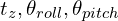$t_{z}, \theta_{roll}, \theta_{pitch}$ as constraints. They have observed a computation reduction of 35% using the 2 step optimization method.

In the featureAssociation.cpp file you will find the edge and planar feature correspondence code in the findCorrespondingCornerFeatures and findCorrespondingSurfFeatures functions. The transformation between edge and planar patches are done in the calculateTransformationCorner and calculateTransformationSurf respectively. As you can see, the transformation calculations of the 6 motion parameters are split between these two functions.

Lidar Mapping

Mapping is the registration of the current scan to the global point cloud map. The global code is represented as $\overline{Q}^{t-1}$ . The L-M method is used here to refine the pose estimation, and the final transformation is obtained from here. Drift estimation is done for this module by performing loop closure detection. In this case, new constraints are added if a match is found between the current feature set and a previous feature set using ICP. The estimated pose of the sensor is then updated by sending the pose graph to an optimization system.

LeGO-LOAM Loop Closure Demo

Explain LOAM paper code in C++ — Figure 10: LeGO-LOAM Loop Closure Demo

The scan2MapOptimization method in the MapOptimization class performs an iterative optimization process to align the current LiDAR scan with the existing map. It first checks if there are sufficient corner and surface points. It then sets up KD-trees for fast nearest-neighbor searches. The method runs up to 10 iterations where it clears previous optimization data, performs corner and surface optimizations to compute residuals and coefficients, and applies the Levenberg-Marquardt algorithm (LMOptimization) to update the transformation parameters. If the optimization converges within these iterations, the loop breaks early. Finally, it updates the transformation parameters based on the optimized values.

void MapOptimization::scan2MapOptimization() {
  if (laserCloudCornerFromMapDSNum > 10 && laserCloudSurfFromMapDSNum > 100) {
    kdtreeCornerFromMap.setInputCloud(laserCloudCornerFromMapDS);
    kdtreeSurfFromMap.setInputCloud(laserCloudSurfFromMapDS);

    for (int iterCount = 0; iterCount < 10; iterCount++) {
      laserCloudOri->clear();
      coeffSel->clear();

      cornerOptimization();
      surfOptimization();

      if (LMOptimization(iterCount) == true) break;
    }

    transformUpdate();
  }
}

Explanation of `main.cpp` :

This code snippet creates and runs a multi-threaded ROS 2 (Robot Operating System 2) executor with four nodes and four threads. The nodes include:

ImageProjection (IP): Projects LiDAR points onto an image plane.
FeatureAssociation (FA): Associates features from the projected image with the current scan and previous scans.
MapOptimization (MO): Optimizes the map using the associated features.
TransformFusion (TF): Fuses transformations from different sources.

The MultiThreadedExecutor allows these nodes to run concurrently on four threads, improving performance by parallelizing their execution. The executor.spin() function keeps the executor running, processing callbacks from the nodes.

The channel.h file defines a template class named Channel that provides a simplistic mechanism for moving information between two threads in a thread-safe manner. This implementation is designed to work with only one writer and one reader, and it is not buffered. The class uses a combination of a mutex (std::mutex), a condition variable (std::condition_variable), and a boolean flag to manage access to the shared resource (_item) between the threads.

ProjectionOut is a structure consisting of two pcl point cloud data and point cloud info message type.

Setup and Run LeGO-LOAM with ROS 2

Below are the steps to run the LeGO-LOAM.

Dependency Management:

To install ROS 2 follow the guide from the article, “setup guide ros2 carla”. Install eigen, boost and gtsam.

Install boost:

# install boost
$ sudo apt install libboost-all-dev # experimented with version 1.74.0

Install Eigen:

# remove eigen if you already have, sudo apt-get remove libeigen3-dev
$ wget https://gitlab.com/libeigen/eigen/-/archive/3.3.7/eigen-3.3.7.zip
$ unzip eigen-3.3.7.zip
$ cd eigen-3.3.7
$ mkdir build && cd build
$ cmake ..
$ sudo make install

Install GTSAM:

$ wget https://github.com/borglab/gtsam/archive/refs/tags/4.2.zip
$ unzip gtsam-4.2.zip
$ cd gtsam-4.2
$ mkdir build && cd build
$ cmake ..
$ sudo make install

Install ROS 2 Dependencies:

$ sudo apt-get install ros-humble-tf2-geometry-msgs ros-humble-tf2-eigen ros-humble-pcl-conversions ros-humble-pcl-ros ros-humble-velodyne ros-humble-velodyne-pointcloud ros-humble-tf2-kdl ros-humble-geometry2 ros-humble-tf2-sensor-msgs ros-humble-tf2-eigen-kdl ros-humble-dummy-robot-bringup ros-humble-rviz2 ros-humble-rviz-default-plugins ros-humble-interactive-markers ros-humble-rviz-common ros-humble-rviz-rendering ros-humble-orocos-kdl-vendor

$ pip3 install rosbags>=0.9.11

Clone LeGO-LOAM:

$ git clone https://github.com/fishros/LeGO-LOAM-ROS2.git

Modify the CMakeLists.txt and LiDAR Topic Name:

This file needs to be modified for easy compilation of the LeGO-LOAM repository. This file can be found at LeGO-LOAM-ROS2/LeGO-LOAM/CMakeLists.txt. there are two modifications,

find_package(Eigen3 REQUIRED) should be changed to find_package(Eigen3 3.3.7 REQUIRED)
Add include_directories(${EIGEN3_INCLUDE_DIR}) after include_directories(include).

To modify the topic name find the file imageProjection.cpp and in the 46th line change /rslidar_points to /velodyne_points.

Either do all the above or download the code from below which is the entire learnopencv code repository. Clone the repository, find this article code folder and just run below commands, given the dependencies are met.

Download Code To easily follow along this tutorial, please download code by clicking on the button below. It's FREE!

Click here to download the source code to this post

$ cd LeGO-LOAM-ROS2
$ colcon build
$ source install/setup.bash

Download the bag file from this link, and this link has the lidar scans that we want to use to perform the LiDAR SLAM using the LeGO-LOAM system. But, right now it’s a ROS 1 bag file, we need to convert it to ROS 2 bag file. to do so run the below command,

$ rosbags-convert nsh_indoor_outdoor.bag

Run the LeGO-LOAM:

# in a seperate terminal
$ ros2 launch lego_loam_sr run.launch.py 

# in a seperate terminal
$ ros2 bag play nsh_indoor_outdoor

LeGO-LOAM ROS 2 code execution

What is LiDAR Odometry and Mapping

Explain LOAM paper code in C++

How to run LOAM on ROS 2

Difference between Visual SLAM and LiDAR SLAM — Figure 11: LeGO-LOAM ROS 2 code execution

Key Takeaways

Important take away from this article are,

Detail understand of the LOAM paper, and how the LiDAR pose is calculated with the detail derivation.
Following up with the LeGO-LOAM paper, which is much advance than LOAM. We went though the the algorithm and how Odometry and Mapping is achieved.
We also covered the code explanation of few parts of LeGO-LOAM.
We finally showed how to run LeGO-LOAM on ROS 2.

Conclusion

The journey from understanding the basic problem of LiDAR SLAM to implementing it in a real-world scenario highlights the complexity and elegance of this field. Whether it’s the meticulous extraction of feature points, the innovative use of ground segmentation in LeGO-LOAM, or the optimization techniques that refine the LiDAR’s pose, each step contributes to creating a precise and reliable map of the environment.

To continue your journey in robotics perception, make sure to check out our other articles in this series, where we cover everything from Monocular SLAM to setting up ROS 2 with Carla. With each post, you’ll build a solid foundation in the key technologies shaping the future of autonomous systems.

References

[ 1 ] LOAM: Lidar Odometry and Mapping in Real-time

[ 2 ] LeGO-LOAM: Lightweight and Ground-Optimized Lidar Odometry and Mapping on Variable Terrain

Introduction to LiDAR SLAM: LOAM and LeGO-LOAM Paper and Code Explanation with ROS 2 Implementation

What is LiDAR SLAM?

Types of Approach to LiDAR SLAM

Paper Summary : LOAM – LiDAR Odometry and Mapping in Real-time

LOAM System Design

Feature Point Extraction

How does the above equation represent a surface smoothness?

How to select feature points?

Feature Correspondences

Estimate the LiDAR Motion

Rodrigues Formula

LiDAR Transformation Calculation

LiDAR Mapping

LeGO-LOAM Paper Summary

Ground Segmentation

Algorithm Implementation:

Feature Extraction

Lidar Odometry

Lidar Mapping

Explanation of `main.cpp` :

Setup and Run LeGO-LOAM with ROS 2

Key Takeaways

Conclusion

References

Get Started with OpenCV

Subscribe to receive the download link, receive updates, and be notified of bug fixes

Which email should I send you the download link?

What is LiDAR SLAM?

Types of Approach to LiDAR SLAM

Paper Summary : LOAM – LiDAR Odometry and Mapping in Real-time

LOAM System Design

Feature Point Extraction

How does the above equation represent a surface smoothness?

How to select feature points?

Feature Correspondences

Estimate the LiDAR Motion

Rodrigues Formula

LiDAR Transformation Calculation

LiDAR Mapping

LeGO-LOAM Paper Summary

Ground Segmentation

Algorithm Implementation:

Feature Extraction

Lidar Odometry

Lidar Mapping

Explanation of main.cpp :

Setup and Run LeGO-LOAM with ROS 2

Key Takeaways

Conclusion

References

Get Started with OpenCV

Subscribe to receive the download link, receive updates, and be notified of bug fixes

Which email should I send you the download link?

Explanation of `main.cpp` :