Recommendation System using Vector Search with Qdrant

Suppose you watched Black Panther on Netflix over the weekend and now want to check out more films like that. When you open Netflix again, it suggests Iron Man, Avengers, and Doctor Strange. This is interesting, right? Why don’t we build something like this? So, in this article, we will build a Recommendation System using Vector Search with Qdrant.

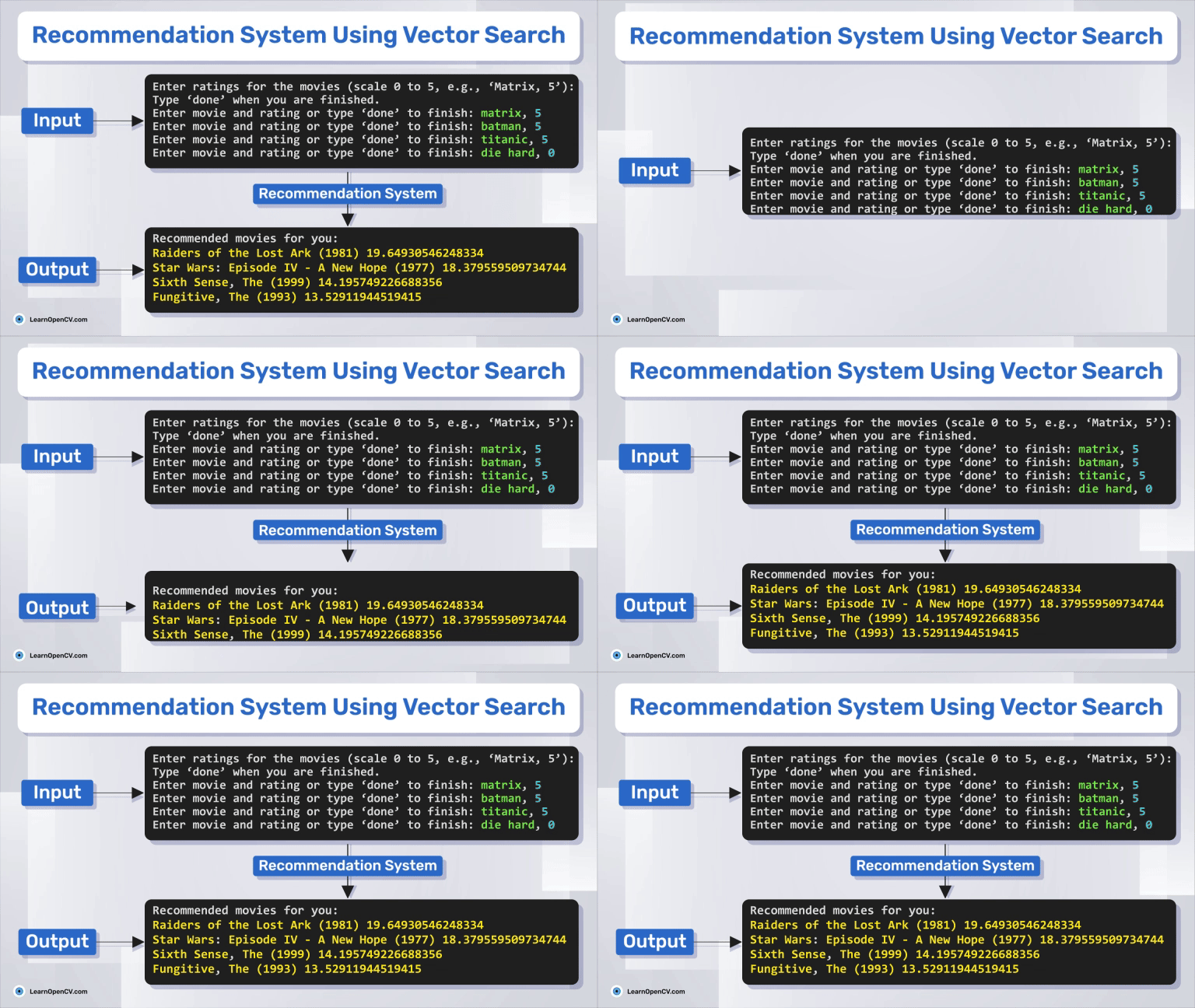
Also, throughout the article, we will discuss:

• What is a recommendation system?
• What is a Vector Database?
• How can RAG improve the traditional recommendation system pipeline?
• How can we build a movie recommendation system using Vector search?
• How does the movie recommendation system work in code?

Cool! Let’s start.

What is a Recommendation System?

A recommendation system is a method or process in which a computer tries to give suggestions like a human. We try to remember in our memory (knowledge base) what may be the perfect choice for another person, as per listening to their expectations and requirements. But how can a machine (computer) do the same?

Here, we developed a set of methods and algorithms that can analyze the relationship between user-item-rating data. As a new user enters, this method (pipeline of algorithms) predicts or recommends items (movies, songs, or products) that the user may like. The journey of the recommendation system started in the late 90s with different traditional approaches like collaborative filtering, TF-IDF, Matrix Factorization, KNN, and Cosine similarity. Then, it improved with Deep Learning methods like CNN, GNN, RAGs, and LLMs throughout the decades. Still, research is going on in this field as it’s part of subjective AI (personalized AI), as humans can hardly identify whether the AI-produced result is right or wrong. Users could be manipulated, utilized, or even cheated by the system. We described the evolution of RecSys in a detailed article, Mastering Recommendation System, for you. You can read it to have a better understanding.

What is a Vector Database?

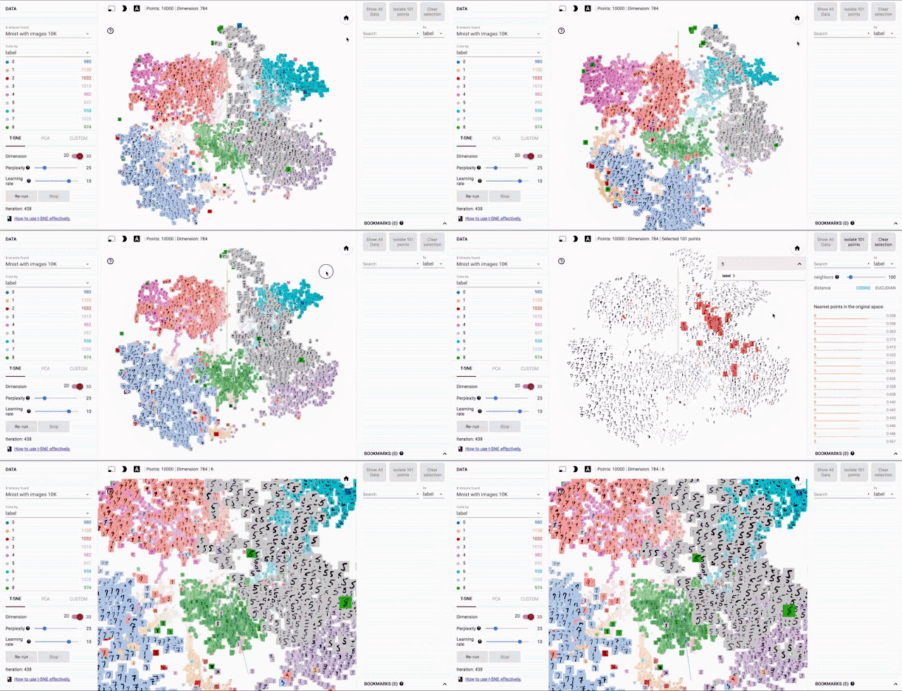
All our advanced AI tasks in NLP or CV heavily depend on embedding (nD Vector representations of text or images). Our traditional databases store strings, numbers, and other scalar data types in rows and columns but cannot work directly when using a multidimensional vector like 3D or 4D tensor. We use a vector database to deal with this type of vector data. A vector database is a specialized database designed to index and store vector embeddings for fast retrieval and similarity search. It has capabilities like CRUD operations, metadata filtering, and vector search.

First, we convert the nD vectors into small embedding chunks and store all the embeddings in a vector database, which helps to make indexing and querying through the vectors more efficient. Some popular Vector DBs are Pinecone, Qdrant, LanceDB, etc.

Now, before proceeding to the main vector database pipeline, we need to know there are two types of vectors:

Sparse vectors

Sparse vectors are all about efficiency and optimization. They store only non-zero elements, making them ideal for data where most values are zero, which is common in natural language processing when dealing with large vocabularies where only a few words might be relevant in any given context. For example, in a document representation, a sparse vector would represent only those words that appear, ignoring all other possible words in the vocabulary. This not only saves a tremendous amount of memory but also speeds up computation since operations are only performed on the non-zero elements.

Consider two documents, each with 200 words. If we employ a sparse vector representation, extracting only the top 2 terms most relevant to the query from each document, our vectors might look like this:

• Document 1 vector: {331: 0.5, … ,14136: 0.7} where ‘331’ and ‘14136’ are indices in a large vocabulary mapping to the words ‘sun’ and ‘moon’.
• Document 2 vector: {764: 0.8, …, 120: 0.4} perhaps representing other key terms like ‘star’ and ‘planet’.

Working with sparse vectors, we can either embed their data with some of their custom methods or use sparse embeddings generated by such sparse methods as Splade (in FastEmbed). These sparse vectors are particularly useful when the dataset is large, and each item (like a document or user profile) involves only a small subset of possible features.

Dense vectors

Dense vectors, on the other hand, are like detailed blueprints—they store values in every dimension, providing a rich and nuanced representation of the data. This makes them suitable for capturing complex relationships and patterns in data, which is essential for tasks like embedding images or detailed text analysis where every element can carry meaningful information.

Using dense vectors for the same two documents might result in each document being represented as an array of several hundred values, most of which would be non-zero:

• Dense Vector Example: [0.2, 0.3, 0.5, 0.7, …, 0.0]

These vectors are generated using deep learning models like BERT for text. These models consider the entire context of the data, thereby capturing a broader representation of features that can be crucial for understanding content deeply.

Amazing right? Want to learn AI and Computer Vision from scratch and build cool projects like these? Join the world’s obviously best AI Courses by OpenCV University. Time is everything, give the best out of you and become the best of yourself.

Vector Database WorkFlow

We can see it as three major steps:

Indexing: After generating the vector embeddings, the vector database indexes vectors using an algorithm like PQ(Product Quantization), LSH(Locality-Sensitive Hashing), or HNSW(Hierarchical Navigable Small World). This step maps the vectors to a data structure that will enable faster searching.

Querying: The vector database compares the input query vector(input query) to the indexed vectors in the dataset to find the nearest neighbors. 

Post Processing: In some cases, the vector database retrieves the k nearest neighbors from the dataset and post-processes them to return the final results. This step can include re-ranking the nearest neighbors using a different similarity measure. We mostly do this step to make a recommendation system using vector search.

Now, when we do the Querying(doing a similarity search), we need a metric to find similarity, right? So we generally use these:

• Cosine similarity: measures the cosine of the angle between two vectors in a vector space. It ranges from -1 to 1, where 1 represents identical vectors, 0 represents orthogonal vectors, and -1 represents vectors that are diametrically opposed. This metric is widely used for various vector types, including sparse and dense representations.

• Euclidean distance: measures the straight-line distance between two vectors in a vector space. It ranges from 0 to infinity, where 0 represents identical vectors, and larger values represent increasingly dissimilar vectors.

• Dot product: measures the product of the magnitudes of two vectors and the cosine of the angle between them. It ranges from -∞ to ∞, where a positive value represents vectors that point in the same direction, 0 represents orthogonal vectors, and a negative value represents vectors that point in opposite directions. This operation is applicable to both dense and sparse vectors.

In this blog, we will use sparse vector search to build our recommendation system. We are using Qdrant as our vector database. We are mostly focused on NLP here, as we are dealing with text data for our recommendation system. However, regarding CV, we can do the similarity search and make recommendations on images, too; read our detailed article about image search with vector database.

How can we use RAG and Vector Search in the Recommendation System Pipeline?

In traditional recommendation systems, we generally use methods like Matrix Factorization or TF-IDF to deal with matrix-based data (like CSV files) that require a lot of data processing, and we can’t directly work with words or sentences (like PDFs), we need to process those into a matrix to work with it. However, after doing all the pre-processing, the recommendations are still not that fast and relevant. But if we can convert our matrix data to vector embeddings, store them in a vector database, and do the similarity search on that vector data, that will be more convenient and easy.  Later, we can integrate an LLM with the recommended data we retrieved and make an entire RAG-based recommendation system.  We can use the RAG pipeline to make recommendations more accurate and faster.

We are using a movie dataset from MovieLens, converting them into sparse vectors using Qdrant and storing them in the qdrant database. We will do a similarity search (vector search) to rank our recommendation. So, we are not using the RAG here but will focus on the retrieval part, and we are using sparse vectors here over the dense vectors for better efficiency and less computational overload. Also, we will do a simple vector search here to perform a retrieval search (so we can think of it as implementing a part of the RAG pipeline). Later on, we have plans to build a recommendation system based on the entire RAG pipeline. Do subscribe to our blog for updates.

Download the Code Here

Click here to download the source code to this post

Code Pipeline

We will follow a very simple approach. Our recommendation system will use collaborative filtering.

The idea behind collaborative filtering is that if two users have similar movie preferences, they will likely to enjoy watching the same movies. We will use this idea to find the users whose ratings are most similar to our own and see what movies these users liked that we haven’t seen yet.

• First, we represent each user’s ratings as a vector in a sparse, high-dimensional space.
• Then, we use Qdrant to store these vectors.
• After that, we find the most similar users to our own ratings using the vector search.
• Finally, we list all movies that similar users liked, which we haven’t seen yet.

We will use the MovieLens Latest Datasets here, a decent and updated dataset. Now, let’s start the coding.

Our code directory has two Python scripts:

RecSys
├── rms.py
└── setup.py

setup.py – to install all the libraries and data.

rms.py – main script for making the recommendations.

First, we create a virtual environment:

conda create -n rms python=3.10.0

We are using miniconda and python 3.10, which are the most stable and easy to use. 

Then, we will activate the environment:

conda activate rms

Now, we will run the setup.py file:

python setup.py

The setup.py file has a very simple code structure:

import os
import subprocess
import sys

def run_command(command):
    """Runs a shell command."""
    result = subprocess.run(command, shell=True, check=True, executable='/bin/bash')
    return result

def install_packages():
    """Installs the required Python packages."""
    try:
        print("Installing required packages using pip...")
        run_command("pip install qdrant-client pandas -q")
        print("Packages installed successfully.")
    except subprocess.CalledProcessError as e:
        print(f"Error installing packages: {e}")
        sys.exit(1)

def create_data_directory():
    """Creates a data directory to store the MovieLens dataset."""
    if not os.path.exists("data"):
        os.makedirs("data")
        print("Created data directory.")

def download_and_extract_data():
    """Downloads and extracts the MovieLens dataset."""
    try:
        print("Downloading MovieLens dataset...")
        run_command("wget https://files.grouplens.org/datasets/movielens/ml-latest-small.zip -q")
        print("Extracting MovieLens dataset...")
        run_command("unzip -q ml-latest-small.zip -d data")
        print("Dataset downloaded and extracted successfully.")
    except subprocess.CalledProcessError as e:
        print(f"Error downloading or extracting dataset: {e}")
        sys.exit(1)

if __name__ == "__main__":
    install_packages()
    create_data_directory()
    download_and_extract_data()

It will install all the required libraries and the dataset. And we are ready with the environment setup. Now, we will go through the rms.py.

Library Import

First, we import the libraries:

import pandas as pd
from qdrant_client import QdrantClient, models
from collections import defaultdict

Initialization of Qdrant Client and Collection

The first step is to initialize the Qdrant client and set up a collection for storing our sparse vectors.

def init_qdrant():
    qdrant = QdrantClient(":memory:")  # Use in-memory for simplicity
    qdrant.create_collection(
        "movielens", vectors_config={}, sparse_vectors_config={"ratings": models.SparseVectorParams()}
    )
    return qdrant

Here, the QdrantClient is initialized with :memory:, which means the data is stored in RAM rather than on disk. This is useful for testing small datasets. We then create a collection named “movielens” in Qdrant. In this collection, we will store the sparse vectors and the movie ratings. We will use the qdrant.create_collection to create the sparse vector collection in our vector database, inside it we use models.SparseVectorParams(), which takes the sparse vectors from our data (the movie ratings). Also, the models class internally uses Pydantic to do all the data modeling and ensure that all parameters and datatypes are in the correct format before passing it to the vector database.

Loading and Normalizing Data

Next, we load the movie data and prepare it for insertion into the Qdrant collection.

def load_data(qdrant):
    tags = pd.read_csv("./data/ml-latest-small/tags.csv")
    movies = pd.read_csv("./data/ml-latest-small/movies.csv")
    ratings = pd.read_csv("./data/ml-latest-small/ratings.csv")

    # Normalize ratings
    ratings.rating = (ratings.rating - ratings.rating.mean()) / ratings.rating.std()

We use pandas to read three CSV files: tags.csv, movies.csv, and ratings.csv. The ratings are normalized by subtracting the mean and dividing by the standard deviation. This standardization process ensures that all ratings are on the same scale, making them easier to compare.

Preparing Sparse Vectors

Once the data is loaded and normalized, we create sparse vectors for each user.

    # Sparse vector preparation
    user_sparse_vectors = defaultdict(lambda: {"values": [], "indices": []})
    for row in ratings.itertuples():
        user_sparse_vectors[row.userId]["values"].append(row.rating)
        user_sparse_vectors[row.userId]["indices"].append(row.movieId)

Our data is vectorized and sparse by nature (ratings of movies by users) and does not need any conversion to embeddings for this task. With a bit of processing, we can directly upload them to our vector database.

Here, we use a defaultdict to store the sparse vectors for each user. For each row in the ratings Dataframe, we add the normalized rating to the values list and the corresponding movieId to the indices list for that user. This creates a sparse representation of each user’s ratings, where only the movies they have rated are included.

Uploading Data to Qdrant

Now that we have the sparse vectors, we need to upload them to Qdrant.

    def data_generator():
        for user in ratings.itertuples():
            yield models.PointStruct(
                id=user.userId, vector={"ratings": user_sparse_vectors[user.userId]}, payload=user._asdict()
            )

    qdrant.upload_points("movielens", data_generator())
    return movies

The data_generator function yields PointStruct objects for each user. Each PointStruct includes the user’s ID, their sparse vector, and additional metadata (payload) from the ratings DataFrame. We then use qdrant.upload_points to insert these points into the "movielens" collection.

Now, if you look at how these sparse vectors are stored in the vector database, this is what you will get:

Total number of users: 610
Total number of key-value pairs: 100836


Uploaded sparse vectors and their shapes from Qdrant:
User ID: 1, Sparse Vector Shape: (232, 232), Sparse Vector: {'values': [0.4781093879267666, 0.4781093879267666, 0.4781093879267666, 1.4373150989349721, 1.4373150989349721, -0.48109632308143896, 1.4373150989349721, . . ., 1.4373150989349721], 'indices': [1, 3, 6, . . ., 3809, 4006, 5060]}
User ID: 2, Sparse Vector Shape: (29, 29), Sparse Vector: {'values': [-0.48109632308143896, . . .,  0.4781093879267666, 1.4373150989349721], 'indices': [318, 333, . . ., 1704, 3578, 6874, 131724]}
.
.
.
User ID: 610, Sparse Vector Shape: (140, 140), Sparse Vector: {'values': [-2.39950774509785, -0.0014934675773361564, 0.4781093879267666, -0.0014934675773361564, 0.4781093879267666, -2.879110600601953, 1.4373150989349721], 'indices': [296, 356, 588, 597, 912, 1028, 1088, 1247, 1307, 1784, 1907, 2571, 2671, 2762, 2858, 2959, 3578, 3882, 4246, 4306, 4447, 4993, 4995, 5066, 5377, 5620, 5943, 5952, 5957]}

The whole thing is HUGE, and this is a small representation for you. In the Qdrant Vector Database (Here movielens) the values(ratings) – indices(movieID) pair for each user stored as a sparse vector. This is what makes the sparse vectors super cool to use for movie recommendations.

Inputting and Normalizing User Ratings

The next function allows a user to input their movie ratings, which are then normalized.

def input_ratings(movies, ratings):
    print("Enter ratings for the movies (scale 0 to 5, e.g., 'Black Panther, 5'):")
    print("Type 'done' when you are finished.")
    final_ratings = {}
    
    mean_rating = ratings.rating.mean()
    std_rating = ratings.rating.std()
    
    while True:
        entry = input("Enter movie and rating or type 'done' to finish: ")
        if entry.lower() == "done":
            break
        try:
            movie_name, user_rating = entry.rsplit(",", 1)
            user_rating = float(user_rating.strip())
            movie_id = movies[movies.title.str.contains(movie_name.strip(), case=False)].movieId.iloc[0]
            
            # Normalize the user's rating
            normalized_input_rating = (user_rating - mean_rating) / std_rating
            print('normalized rating:', normalized_input_rating)
            final_ratings[movie_id] = normalized_input_rating
        except IndexError:
            print(f"Movie '{movie_name.strip()}' not found in the database. Please try again.")
        except ValueError:
            print("Please enter a valid rating between 0 and 5.")
    
    return final_ratings

This function prompts the user to input ratings for movies. It first extracts the movie name and rating from the user’s input, then finds the corresponding movieId from the movies DataFrame. The rating is normalized to fit within the range of -1 to 1. The resulting dictionary contains movie IDs as keys and normalized ratings as values.

Generating Movie Recommendations

Finally, we generate movie recommendations based on the user’s input.

def recommend_movies(qdrant, movies, my_ratings):
    def to_vector(ratings):
        vector = models.SparseVector(values=[], indices=[])
        for movieId, rating in ratings.items():
            vector.values.append(rating)
            vector.indices.append(movieId)
        return vector

    results = qdrant.search(
        "movielens",
        query_vector=models.NamedSparseVector(name="ratings", vector=to_vector(my_ratings)),
        with_vectors=True,
        limit=20,
    )

    movie_scores = defaultdict(lambda: 0)
    for user in results:
        user_scores = user.vector["ratings"]
        for idx, rating in zip(user_scores.indices, user_scores.values):
            if idx in my_ratings:
                continue
            movie_scores[idx] += rating

    top_movies = sorted(movie_scores.items(), key=lambda x: x[1], reverse=True)
    print("Recommended movies for you:")

    for movieId, score in top_movies[:5]:
        print(movies[movies.movieId == movieId].title.values[0], score)

The recommend_movies function is the heart of the code. Here, we try to make personalized movie recommendations using the power of sparse vectors and the Qdrant vector search engine. First, it transforms the movie ratings we provided into a sparse vector with the to_vector function. Here, it creates a SparseVector object whose corresponding index and rating value represent each movie we rated. Next, we use this sparse vector, wrapped in a NamedSparseVector, to do the vector search in our movielens collection (Our local Vector DB), looking for users who have similar tastes. Using the qdrant.search, the function queries the vector database to find other user vectors that are similar to the input user vector (Top-K similarity scores calculated from dot product between query ratings(vector) and stored ratings (vector)). And here is how it looks when Qdrant gives the recommendation TopK vectors:

ScoredPoint(id=514, version=0, score=-0.6886219382286072, payload={}, vector={'ratings': SparseVector(indices=[1, 11, 16, 22, 34, 44, 47, 62, 150, 161, 162, 185, 260, 261, 296, 339, 356, 364, 440, 457, 474, 480, 586, 588, 589, 592, 593, 595, 596, 597, 608, 648, 778, 785, 919, 1022, 1036, 1079, 1089, . . ., 184931, 184987, 185029, 185033, 185473, 185585, 186587, 187031, 187593, 187595, 188797], values=[0.4781093879267666, 0.4781093879267666, -0.0014934675773361564, -0.48109632308143896, 0.4781093879267666, -0.9606991785855417, . . ., 0.4781093879267666, 0.4781093879267666, 0.4781093879267666, 0.4781093879267666, 0.4781093879267666])}, shard_key=None, order_value=None)
 ScoredPoint(id=567, version=0, score=-0.9179245233535767, payload={}, vector={'ratings': SparseVector(indices=[1, 34, 50, 101, 260, 308, 356, 364, 480, 541, 648, 673, 750, 903, 924, 954, 1196, 1197, 1198, 1203, . . ., 176371, 176419, 177765, 178827, 179491, 179749, 179815, 179819, 180031, 180985, 182823, 183897, 184253], values=[-0.0014934675773361564, -0.9606991785855417, -2.39950774509785, . . ., -0.48109632308143896, -1.4403020340896444, -0.9606991785855417, -0.48109632308143896, -0.9606991785855417])}, shard_key=None, order_value=None)]

We then look into these results vectors, pulling out the ratings from movies we haven’t rated yet but that were highly rated by users with similar preferences. These new ratings get aggregated into a movie_scores dictionary, where each movie’s ID is mapped to a cumulative score based on the ratings it received from similar users. Importantly, we skip over any movies that we already rated, ensuring that our recommendations are fresh. Finally, we sort these movies by their scores in descending order, bringing the top-rated recommendations right to the forefront. We then print out the top five movies, along with their scores, to give you a set of personalized movie recommendations based on the tastes of others who share your viewing habits.

Let’s consider a small example: we provided an input vector like this

my_ratings: indices=[5, 11, 18, 22, ..], values=[0.478, -0.481, 0.957, 0.478, ..]

Where the indices are the movieID and values are the ratings. Then, after we do the similarity search, the vector database gives similar user vectors (user vectors contain few similar movieID-ratings pairs in it) like this:

# SparseVector indices for various movies with associated ratings.

ScoredPoint 1: indices=[1, 11, 16, 22, ..], values=[0.478, -0.481, 0.957, 0.478, ..]
ScoredPoint 2: indices=[1, 34, 18, ..], values=[-0.001, -0.960, -2.399, ..]

Now, It’s very simple processing for us:

Aggregation of Scores

• Loop Through Each User (ScoredPoint):
  • For ScoredPoint 1:
    • Check each index and rating:
      • If index 1 is not in my_ratings, add 0.478 to its score in movie_scores.
      • Continue this for indices 11, 16, and 22, adding their respective ratings to movie_scores.
  • For ScoredPoint 2:
    • Similar logic:
      • If index 1 is not in my_ratings, add -0.001 to its existing score (it’s now 0.478 - 0.001 = 0.477).
      • Continue for indices 34 and 18.

Sample Calculation:

We haven’t rated the movieID-1 movie, but both the similar taste users rate that one here, so it’s a fresh recommendation for us. The aggregation for index 1 across both users would be:

movie_scores[1] = 0.478 (from user 1) - 0.001 (from user 2) = 0.477

Similarly, aggregation scores for other indices, like 11, 16, 22, 34, and 18 would be calculated based on the respective ratings provided by each user in the result set (if applicable). And we will get a bunch of fresh recommended movies in our bucket.

Sorting for Recommendations

• Sort by Scores:

top_movies = sorted(movie_scores.items(), key=lambda x: x[1], reverse=True) 

This will rank the movies by their total aggregated scores. Higher scores suggest more positive feedback from users with similar tastes. Cool right! We made it; the recommendation system is ready for work.

Main Execution

The final part of the code ties everything together:

if __name__ == "__main__":
    qdrant = init_qdrant()
    movies = load_data(qdrant)
    my_ratings = input_ratings(movies)
    recommend_movies(qdrant, movies, my_ratings)

This block first initializes Qdrant and loads the data into the collection. It then collects the user’s movie ratings and generates personalized recommendations based on those ratings. This workflow ensures that the system is set up and ready to provide recommendations in a smooth and logical sequence.

Experimental Results

Let’s have a look at the results now: 

We will input a few movies with a rating (0 to 5) according to our likes and dislikes:

Enter ratings for the movies (scale 0 to 5, e.g., 'Black Panther, 5'):
Type 'done' when you are finished.
Enter movie and rating or type 'done' to finish: Black panther, 4
normalized rating: 0.4781093879267666

And we get our fresh movie recommendations like this:

Recommended movies for you:
Spider-Man: Homecoming (2017) 8.138313867796384
Logan (2017) 7.66319141502429
Guardians of the Galaxy 2 (2017) 7.660204479869619
WALL·E (2008) 7.660204479869617
Thor: Ragnarok (2017) 7.660204479869617

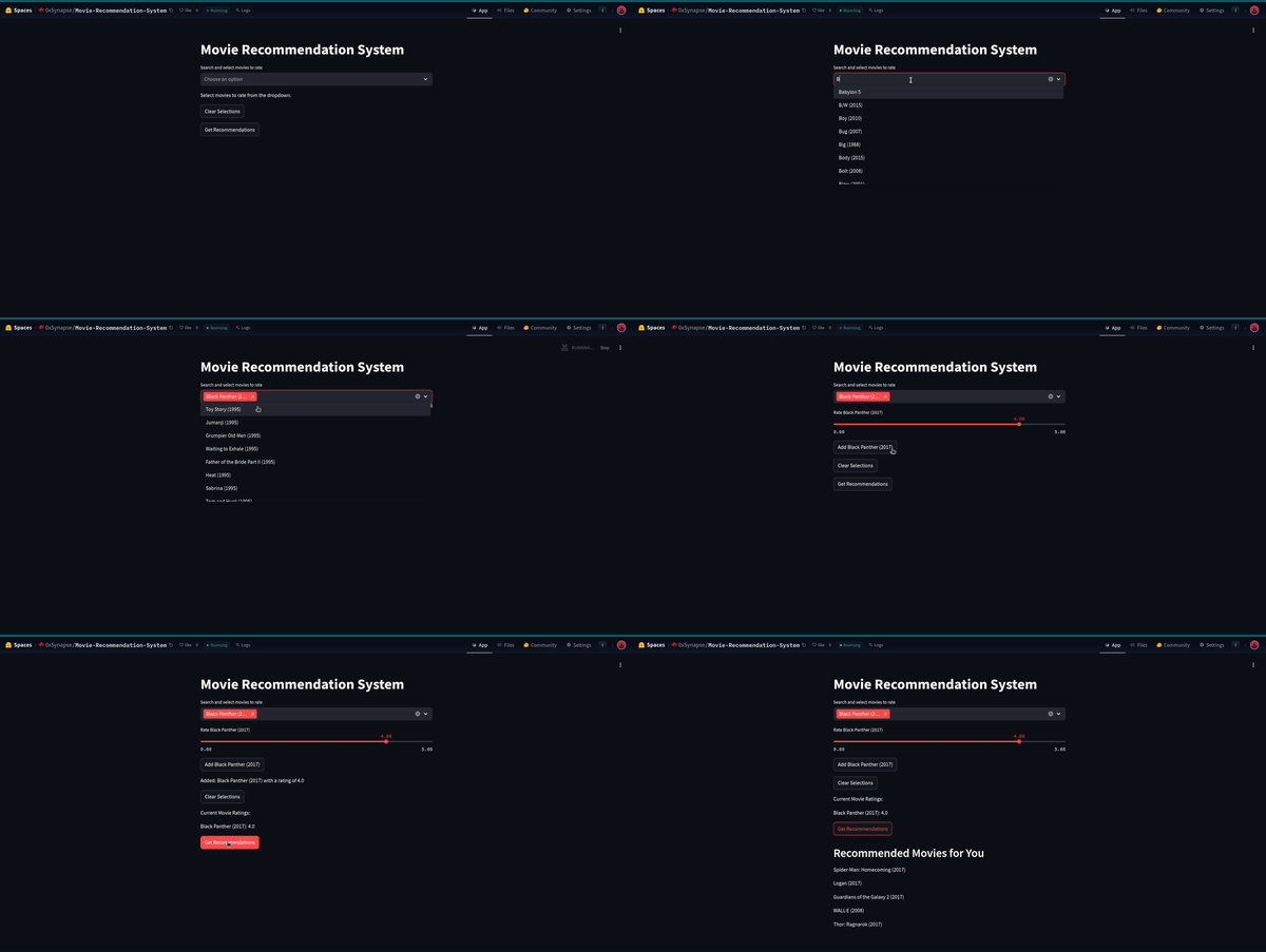
Also, we made a streamlit app for you to go and play with it:

Key Takeaways

Vector Databases for Recommendations: The article explains how vector databases like Qdrant are used to store and retrieve high-dimensional vector embeddings, which are crucial for performing similarity searches in recommendation systems. These databases enable efficient indexing and querying of vector data, improving the performance of recommendation engines.

Sparse v/s Dense Vectors: The article distinguishes between sparse and dense vectors. Sparse vectors come in handy when most of your data elements are zeros. They’re like the minimalist approach to data storage, keeping track of only the non-zero values and where they’re located. This approach is a real space-saver, especially with huge datasets where many features don’t appear often, like in text analysis. On the flip side, dense vectors are typically full of non-zero values. Every element is explicitly stored, which means that no matter the value, each position in a dense vector holds data that needs to be recorded. This makes dense vectors straightforward but can eat up more memory.

RAG Pipeline for Improved Recommendations: This article discusses how we can implement the entire Retrieval-Augmented Generation (RAG) pipeline to make recommendations more accurate and relevant. We explored how the recommendation process becomes more accurate and efficient by converting matrix data to vector embeddings, storing them in a vector database, and performing similarity searches. We also planned to build an entire RAG-based recommendation system in one of our future articles.

Code Implementation of Recommendation System: The article demonstrates how to implement a movie recommendation system using collaborative filtering. By representing user ratings as sparse vectors, indexing them in Qdrant, and performing vector searches, the system identifies users with similar tastes and recommends movies based on their preferences.

Conclusion

And that’s a wrap! We hope you now feel confident in creating your own recommendation system using vector search. With the knowledge you’ve gained, you should be able to build a simple and efficient recommendation engine like a Spotify clone.

We’d love to hear about any cool projects you build; feel free to share your experiences and insights with us!

References

1. Qdrant Documentation
2. Pydantic Documentation
3. Image Source – Spotify R&D, Medium