Anchor free object detection is powerful because of its speed and generalizability to other computer vision tasks. “CenterNet: Object as Points” is one of the milestones in the anchor-free object detection algorithm. In this post, we will discuss the fundamentals of object detection, anchor free (anchorless) vs. anchor-based object detection, CenterNet Object as Points paper, CenterNet pose estimation, and inference of the CenterNet model.
| The objective of the blog post is to answer the following questions. 1. What is object detection in Machine Learning/Deep Learning? 2. What is an anchor in object detection? 3. What is anchor-based object detection? 4. What is anchor-free object detection? 5. Is anchor free better than anchor-based object detection? |
People who will benefit most from this article are those who:
- Understand the deep learning classification pipeline and want to learn deep learning-based object detection.
- Have experience in anchor-based object detection and want to explore anchor free object detection.
- Want to dive deep into CenterNet Object as Points algorithm.
- Want to access models from the TensorFlow model zoo and use it in your application.
- What is Object Detection in Machine Learning/Deep Learning?
- What is an Anchor in Object Detection?
- What is Anchor-Based Object Detection?
- What is Anchor-Free Object Detection?
- Is Anchor-Free Better Than Anchor-based Object Detection?
- Components of Deep Learning-Based Object Detection
- How Does CenterNet Work?
- Ground Truth Encoding in CenterNet
- Model Prediction Decoding in CenterNet
- Loss Functions in CenterNet
- CenterNet Pose Estimation
- CenterNet model Inference using TensorFlow
- Conclusion
What is Object Detection in Machine Learning/Deep Learning?
Object detection is a computer vision technique to localize and classify objects in an image or video. The deep learning-based object detection technique is highly successful with many applications using object detection, for example, surveillance and tracking.
What is an Anchor in Object Detection?
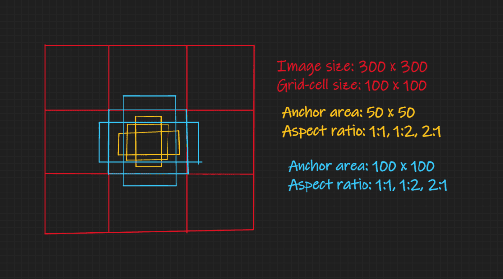
Pre-defined bounding boxes as proposals of the ground truth are called anchors in object detection. Let us understand it by an example.

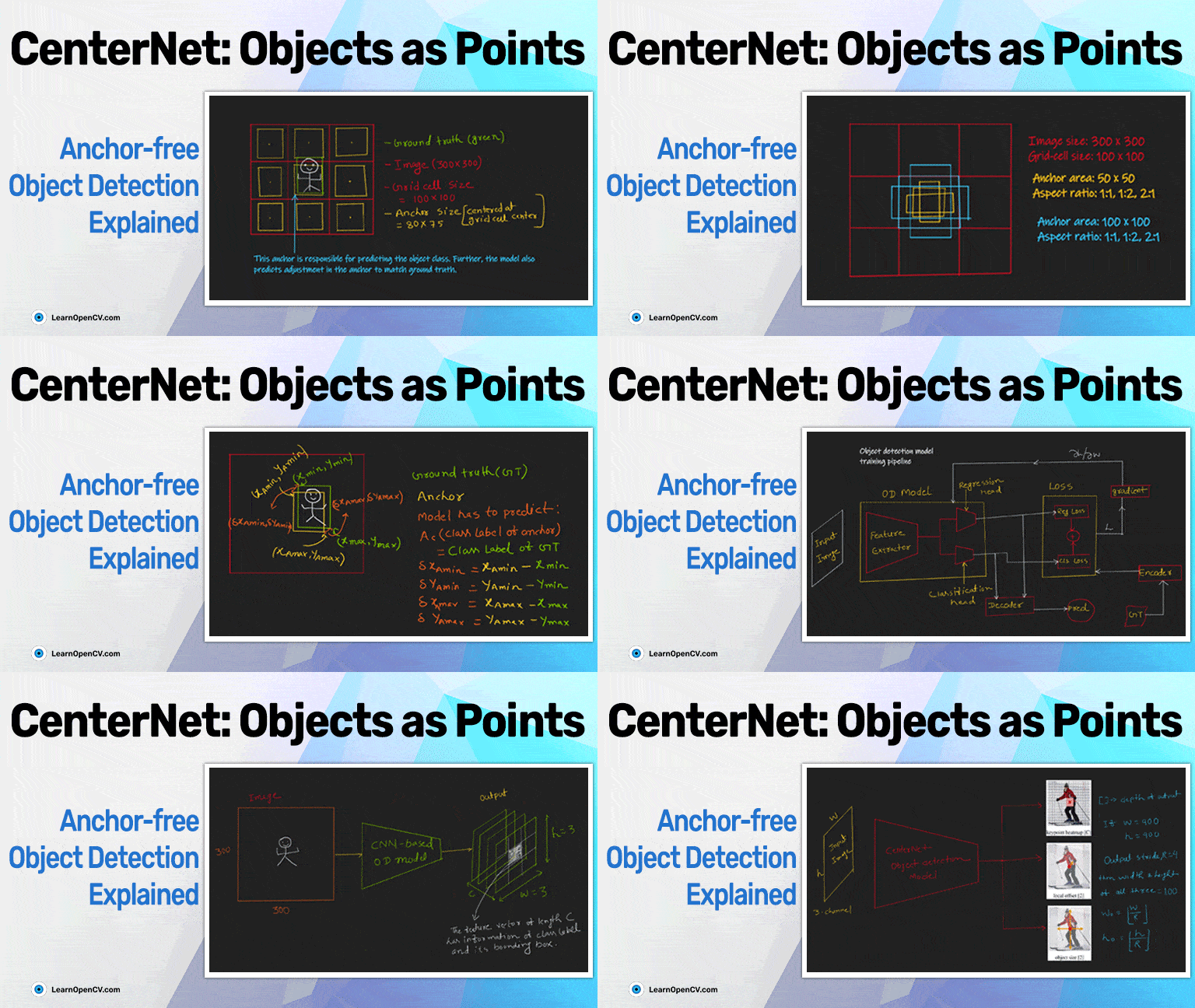
Suppose you have an image of the size 300 x 300 as shown above (fig. 1). It is equally divided into 3 x 3 grid cells. A bounding box of size 80 x 75 is at the center of each grid cell. These predefined bounding boxes (yellow color) are called anchors. If any of these proposals have enough overlap with the ground truth bounding box, then it will be assigned the ground truth’s class labels, else it will be assigned background class labels (no object class labels).
One grid cell may have multiple pre-defined bounding boxes/proposals, as shown in the below image. (fig. 2).
What is Anchor-Based Object Detection?
A deep learning-based object detection method that uses pre-defined bounding boxes (anchors) as proposals is known as anchor-based object detection.
Anchors are assigned class labels with a label assignment strategy. For example, in a naive label assignment strategy, if the maximum IoU (Intersection over Union) of an anchor with some ground truth is greater than 0.5, then the anchor will be assigned the ground truth label.
In anchor-based object detection, the model predicts the class labels of anchor boxes and how the anchor should be adjusted to match it with ground truth objects as below. (fig. 3).

What is Anchor Free Object Detection?
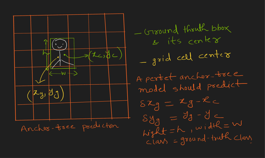
Anchor free object detection directly predicts the bounding box, but it predicts it with respect to some fixed reference in the image.
For example, consider an image of size 300 x 300 as below (fig. 4). It is equally divided into 6 x 6 grid cells. The ground truth center will fall in one of the grid cells. Therefore, only the grid cell is responsible for predicting the object’s width, height, and center deviation from the grid cell center.
Is Anchor Free Better Than Anchor-based Object Detection?
The initial success of the anchor-based method led to more research, which made it more accurate than anchor free object detection. However, recent success in anchor free object detection made it equivalent to the anchor-based method in terms of accuracy.
Following are a few advantages of anchor free methods over anchor-based:
- Finding suitable anchor boxes (in shape and size) is crucial in training an excellent anchor-based object detection model. Finding suitable anchors is a complex problem and may need hyper-parameter tuning.
- Using more anchors results in better accuracy in anchor-based object detection but using more anchors comes at a cost. The model needs more complex architecture, which leads to slower inference speed.
- Anchor free object detection is more generalizable. It predicts objects as points that can easily be extended to key-points detection, 3D object detection, etc. However, the anchor-based object detection solution approach is limited to bounding box prediction.
Components of Deep Learning-Based Object Detection
Before discussing how CenterNet object detection works, let’s look at how deep learning-based object detection generally works.
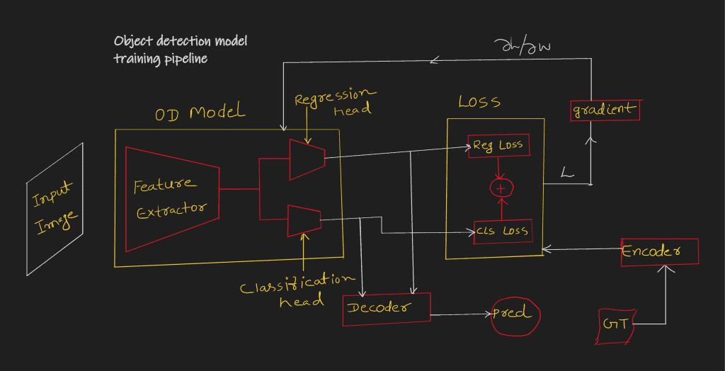
Object detection has the following four components (fig. 5):
- Object detection model
- Ground truth encoding
- Loss function
- Model prediction decoding
Object Detection Model
A CNN (Convolution Neural Network) based architecture that maps input images to low-resolution features. These features have rich information about objects (object localization and its class) of the image (fig. 6).

However, a simple CNN architecture is less effective for an object detection task because deeper layers output (starting from input) lack localization information. FPN [3] or similar architecture solves this problem. We will discuss this in a future post.
Ground Truth Encoding in Object Detection
To compare the model output and ground truth label using some loss, both should be of the same shape.
In fig. 6 (above), you can see that the model output size is ![]() . However, the ground truth labels for an image have the following (or similar) format:
. However, the ground truth labels for an image have the following (or similar) format:
![]()
So for training, it is essential to convert these labels into the model output format. Converting ground truth in a specific format is called ground truth encoding.
Loss Function in Object Detection
Object detection model training also needs a loss function like other neural network training.
An object detection problem has two parts:
- Localization of an object (predicting four numbers to represent a bounding box) is a regression problem.
- Predicting the class label of the localized coordinate is a classification problem.
So it needs two different loss functions to solve these two problems. The weighted sum of localization and classification loss is the final loss of the object detection model prediction.
The number of background classes is much higher than the object class, which makes the object detection problem harder. So it needs a classification loss function that can deal with skewed data, for example, focal loss [4].
Object Detection Model Prediction Decoding
The model output needs to be decoded (reverse of ground truth encoding) to ground truth format, (![]() ).
).
Now that you know the deep learning-based object detection components let us see how CenterNet implements these components.
How Does CenterNet Work?
Before going further, it is essential to know the timeline of CenterNet. In April 2019, the following two papers were published in CVPR:
- Object as Points by Xingyi Zhou, Dequan Wang, Philipp Krähenbühl [1]
- CenterNet: Keypoint Triplets for Object Detection by Kaiwen Duan, Song Bai, Lingxi Xie, Honggang Qi, Qingming Huang, Qi Tian [2]
In the paper “CenterNet: Objects as Points,” the authors use the term CenterNet to refer to their algorithm. Let us go through the following aspects to understand how CenterNet works.
- Ground truth encoding
- Model prediction decoding
- Model prediction decoding
- CenterNet Model (backbone architecture)
Ground Truth Encoding in CenterNet
In CenterNet, an object is modeled as the center point of its bounding box. The bounding box size and other object properties are inferred from the keypoint feature at the center (fig. 7).

Ground truth encoding depends on the object detection model output. So, first, let us look at the model output (fig. 8).
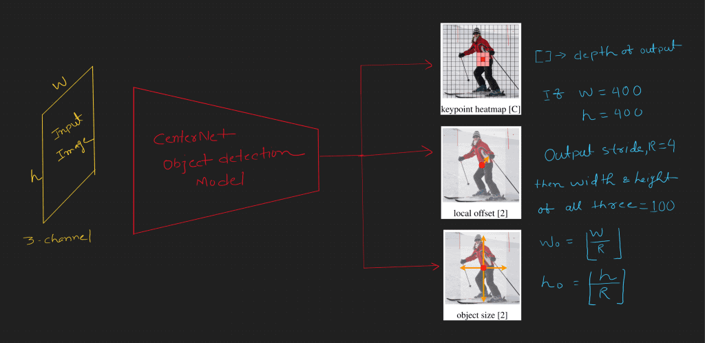
The model has three output heads: the keypoint heatmap, object size, and local offset. First, it takes an input image of shape ![]() . The output stride is
. The output stride is ![]() , so the output width and height are
, so the output width and height are ![]() and
and ![]() , respectively. And what about the depth (channels) of each output head? The depth of the keypoint heatmap is
, respectively. And what about the depth (channels) of each output head? The depth of the keypoint heatmap is ![]() (number of object classes), the object size is
(number of object classes), the object size is ![]() , and the local offset is
, and the local offset is ![]() . Let’s look at why this is so.
. Let’s look at why this is so.
Keypoint Heatmap in CenterNet
It has one channel for each object class. So the depth is the number of an object class (e.g., 80 for the COCO dataset). The keypoint heatmap is responsible for keypoint encoding and prediction.
How is the CenterNet keypoint heatmap encoded?
Let us assume a point ![]() ,
, ![]() is the center of a bounding box. The output stride of the CenterNet model is
is the center of a bounding box. The output stride of the CenterNet model is ![]() , so the point in the heatmap space will be
, so the point in the heatmap space will be ![]() ,
, ![]() (let).
(let).
The ground truth encoding (keypoint value, at ![]() for class
for class ![]() ),
), ![]() in the heatmap space is assigned using Gaussians kernel as follows:
in the heatmap space is assigned using Gaussians kernel as follows:
(1) ![]()
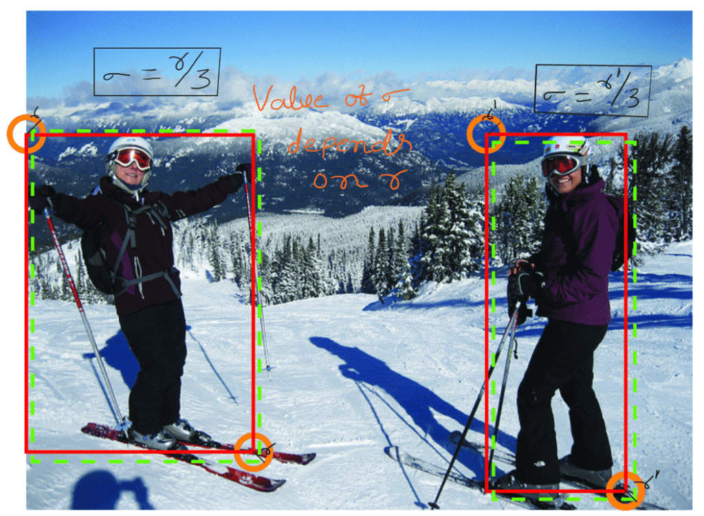
Here, ![]() is the object size-adaptive standard deviation. It means
is the object size-adaptive standard deviation. It means ![]() depends on the bounding box shape and size. How do we calculate it? Have a look at the following image (fig. 9).
depends on the bounding box shape and size. How do we calculate it? Have a look at the following image (fig. 9).
(2) ![]()
where ![]() is the radius.
is the radius.
Find the radius as follows:
- Assume a circle of radius
 on the top-left and bottom-right corner of a bounding box.
- The largest possible radius that satisfies the property: Any pair of points, one from the top-left circle and the other from the bottom-right circle, generate the bounding box (dotted green line) with at least
 IoU with ground truth (solid red line).
Look at heatmap values around the bounding box center in heatmap space (fig. 10).
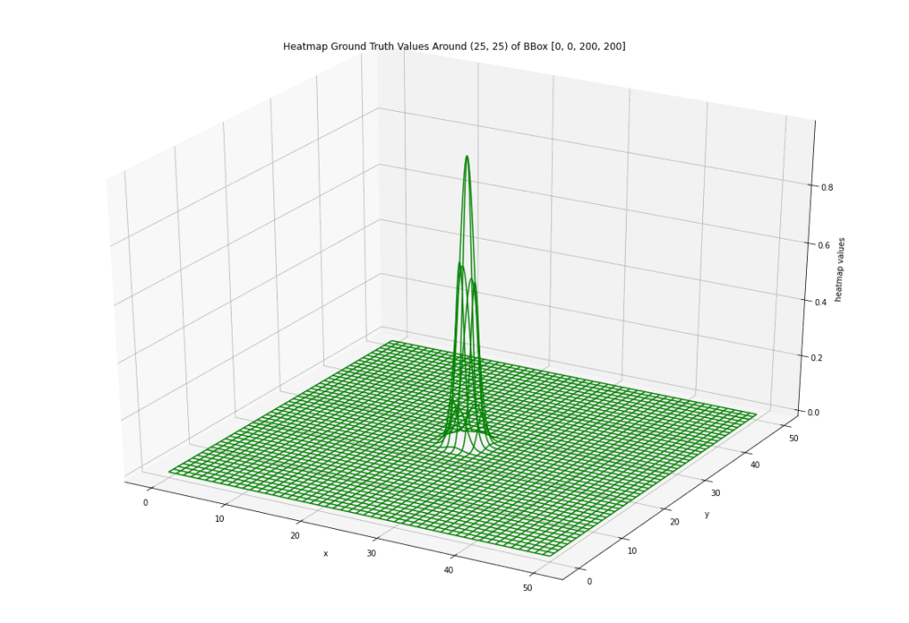
What if the image has more than two instances of the same class? In this case, ![]() will take the maximum value of all.
will take the maximum value of all.
Local Offset in CenterNet
Mapping to the heatmap space, the points lose their precision because of the CenterNet model output stride, ![]() .
.
For example, if a point, ![]() , is in the original image space.
, is in the original image space.
In heatmap space (let’s ![]() ), the point will be
), the point will be ![]() .
.
If one remaps it to the original image space only using ![]() , the point remaps to
, the point remaps to ![]() .
.
For the ![]() -coordinate, there is an error of
-coordinate, there is an error of ![]() pixels.
pixels.
To fix such errors, the model also predicts the local offset of the heatmap points. So it has two channels for improving the ![]() -coordinate and
-coordinate and ![]() -coordinate.
-coordinate.
The ground truth encoding of offset for point p_tilde is the following:
(3) ![]()
Using the offset, you can obtain the precise point in the original image. Let us review the above example.
![]()
![]()
Re-maps to the original image space:
![]()
It gets the original point ![]() in the image using offset value and heatmap.
in the image using offset value and heatmap.
Object Size in CenterNet
It predicts the width and height of the bounding box, so its depth is two.
How do we achieve ground truth encoding for object size?
Let ![]() be a bounding box of the class label,
be a bounding box of the class label, ![]() , in the original image space.
, in the original image space.
So the center point in image space is:
![]()
It’s center point, ![]() in the model output space (stride,
in the model output space (stride, ![]() ) is:
) is:
![]()
Then, the object size label (encoding) in the model output space, ![]() , is:
, is:
(4) ![]()
Width and height encoding is only needed for bounding box centers. However, the model will predict values for other points as well. Predictions other than the bounding box center will not contribute to training.
Model Prediction Decoding in CenterNet
Decoding is the reverse of encoding. The final prediction will be a combination of all three head outputs combination.
- Heatmap prediction,
- Offset prediction, and
- Size prediction
Heatmap for bounding box center (keypoint): The point at which all eight neighboring points have a lower value becomes a potential point for the bounding box center (key point). Select the top ![]() points to form each channel (for each class).
points to form each channel (for each class).
Offset for bounding box center correction: Once the potential locations are found from the heatmap, it will be corrected using offset prediction.
For example, If a heatmap point is ![]() and offsets prediction at
and offsets prediction at ![]() is
is ![]() and assume the output stride,
and assume the output stride, ![]() .
.
So the center in the image space will be ![]() .
.
Size of bounding box width and height prediction: For each selected point on the heatmap, size prediction will give the width and height of the bounding box.
Loss Functions in CenterNet
As the CenterNet model has three output heads, it also needs three loss functions.
- Heatmap Loss
- Offset Loss
- Object Loss
Let us use the same notations in ground truth encoding. Let us denote the corresponding prediction with hat (^).

Heatmap Loss:
(5) 
Where ![]() is a number of bounding boxes (key points).
is a number of bounding boxes (key points).
![]() and
and ![]() are hyper-parameters of the focal loss.
are hyper-parameters of the focal loss.
The first part, where ![]() :
:
![]()
It is a focal loss for positive class.
Focal loss is a modified version of cross-entropy loss ![]() where it discounts the cross-entropy loss by a factor
where it discounts the cross-entropy loss by a factor ![]() . You can notice that if
. You can notice that if ![]() is close to zero then
is close to zero then ![]() is close to one. So the loss is significantly less. However, if
is close to one. So the loss is significantly less. However, if ![]() is high, then
is high, then ![]() becomes very small, then the loss discounts are heavy
becomes very small, then the loss discounts are heavy
In other words, the loss contribution from confident prediction is much less compared to a not-confident one.
Hence focal loss is powerful in dealing with class imbalance.
The second part: where, ![]()
![]()
Let’s break it into two:
- The focal loss component for negative class:

- The multiplying factor:

The first part is a focal loss for the negative class.
The second multiplying factor ![]() is a discounting factor of negative class focal loss. The value of
is a discounting factor of negative class focal loss. The value of ![]() is high (close to one) near the bounding box center. So the value of
is high (close to one) near the bounding box center. So the value of ![]() is small near the bounding box center, and
is small near the bounding box center, and ![]() increases as it goes away from the bounding box center. This means that points near the bounding box center are less negative than those farther.
increases as it goes away from the bounding box center. This means that points near the bounding box center are less negative than those farther.
Offset Loss: For offset, it uses mean absolute error (MAE).
(6) ![]()
It calculates loss only at the bounding box center (keypoints) in output space.
Object loss: It also uses the mean absolute error (MAE).
(7) ![]()
It calculates loss only at the bounding box center (keypoints) in output space. Other points do not have width and height labels.
CenterNet Model (Backbone Architecture)
CenterNet uses three different backbones in their experiments (fig. 11):
- ResNet
- Deep Layer Aggregation (DLA)
- A Stacked Hourglass

ResNet and DLA are modified. In addition, up-convolution is added to increase the output resolution. Finally, deformable convolution is added to make the model more robust to geometric variation of objects.
CenterNet Pose Estimation
Before seeing how CenterNet solves pose estimation, let us restate how it solved the object detection problem.
CenterNet is predicting the following to solve object detection problem:
- Heatmap: Each class has one channel to predict the corresponding class’s key points. Here key points are bounding box center.
- Offset: Further, offset fixes key points’ precision.
- Object size: It predicts two features, the object’s width and height at its bounding box center.
Have a look at the image below (fig. 12).
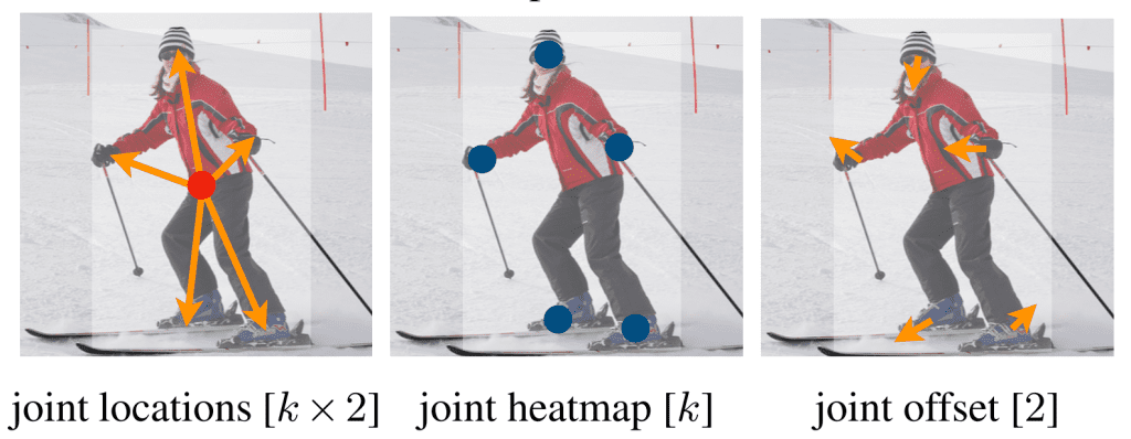
Joint Heatmap: Let us assume ![]() joints as different class labels in the pose estimation. So heatmap needs
joints as different class labels in the pose estimation. So heatmap needs ![]() -channels to predict these classes.
-channels to predict these classes.
Joint Offset: It improves the precision of joints’ key points.
Joint Locations: It predicts the locations of joints from the object center. To represent ![]() points in
points in ![]() space, it needs
space, it needs ![]() numbers. So it predicts
numbers. So it predicts ![]() features at the object center.
features at the object center.
The above explanation is about encoding/prediction. What about decoding?
It gets key points from the heatmap, which exceeds a threshold value of, say, ![]() .
.
Key points with respect to the object center are also predicted in joint locations.
These two predictions are mapped using minimum distance for each class. However, the heatmap prediction is the final prediction. So essentially, this exercise is to find the map key points to its object center.
Finally, you have the object center, and key points belong to the object center, which completes the decoding.
CenterNet Results
Speed vs. Accuracy Plot (fig. 13):
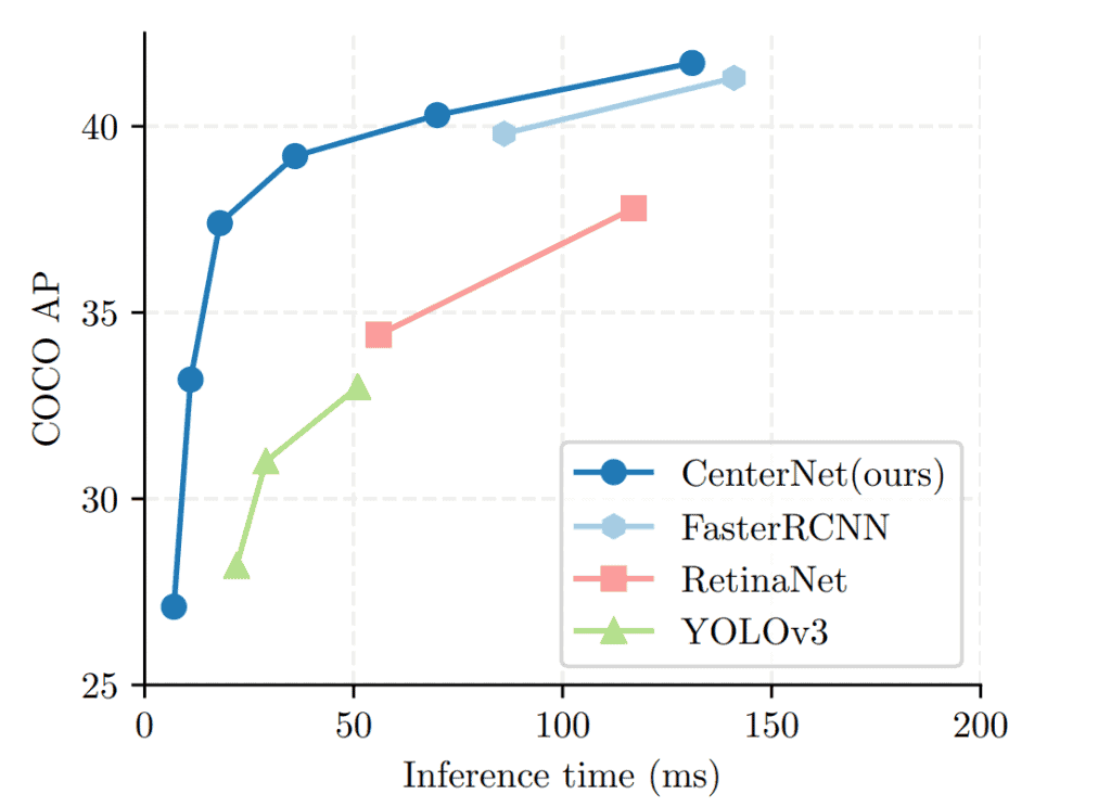
Speed-accuracy trade-off for real-time detectors. CenterNet outperforms a range of state-of-the-art algorithms.
Below is the speed-accuracy trade-off of different CenterNet models (fig. 14).

Here, AP is Average Precision.
It uses three augmentations for AP calculation:
- Inference with the original image (NA).
- Inference with the original and flipped images, the final prediction is average to two predictions (F).
- Inference with the original flipped and multiscale resolution, the final prediction uses NMS (MS).
The FPS reports are with image size 512 x 512 on TITAN-V GPU.
Sample Prediction
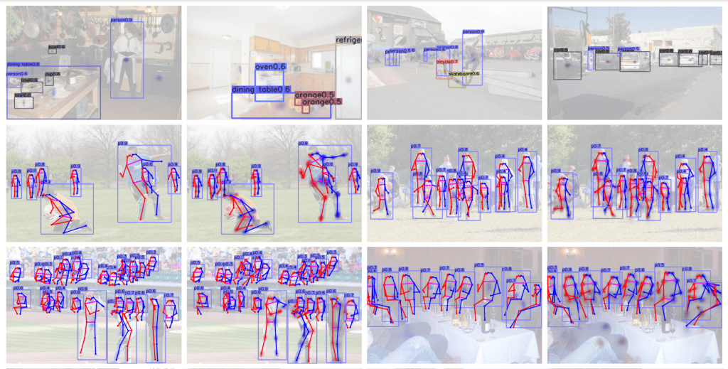
Below is the prediction from the CenterNet model for object detection (1st row) and pose estimation (2nd and 3rd row) (fig. 15).
CenterNet model Inference using TensorFlow
The authors have provided the code on GitHub [6]. However, we will use TensorFlow Hub [7] to download the pre-trained CenterNet models and make inferences.
import cv2
import numpy as np
import tensorflow as tf
import tensorflow_hub as hub
import matplotlib.pyplot as plt

import urllib
Select CenterNet Models
TensorFlow hub has the following CenterNet pre-trained model:
- ResNet18
- ResNet50
- ResNet101
- DLA-34
- Hourglass104
Here, we will use ResNet101 and Hourglass104 for inference.
models = {
          'Resnet101':'https://tfhub.dev/tensorflow/centernet/resnet101v1_fpn_512x512/1',
          'HourGlass104':'https://tfhub.dev/tensorflow/centernet/hourglass_512x512/1'
         }
Download Images
Images URLS.
images = [
          'https://farm7.staticflickr.com/6073/6032446158_85fa667cd2_z.jpg',
          'https://farm9.staticflickr.com/8538/8678472399_886f8eabec_z.jpg',
          'https://farm6.staticflickr.com/5485/10028794463_d8cbb38932_z.jpg',
          'https://farm4.staticflickr.com/3057/2475401198_0a342a907e_z.jpg'
         ]
Download images.
# Download images.
for i in range(len(images)):
    urllib.request.urlretrieve(images[i], "img{}.jpg".format(i+1))
Read images.
# Read Images.
img1 = cv2.imread('img1.jpg')
img2 = cv2.imread('img2.jpg')
img3 = cv2.imread('img3.jpg')
img4 = cv2.imread('img4.jpg')
Plot images.
def plot_images(img_list, title=None, row=1, column=2,
                fig_size=(10, 15)):
    plt.figure(figsize=fig_size)
    for i, img in enumerate(img_list):
        plt.subplot(row, column, i+1)
        plt.imshow(img[...,::-1])
        plt.axis('off')
        plt.title(title[i] if title else 'img{}'.format(i+1))
    plt.show()
image_list = [img1, img2, img3, img4]
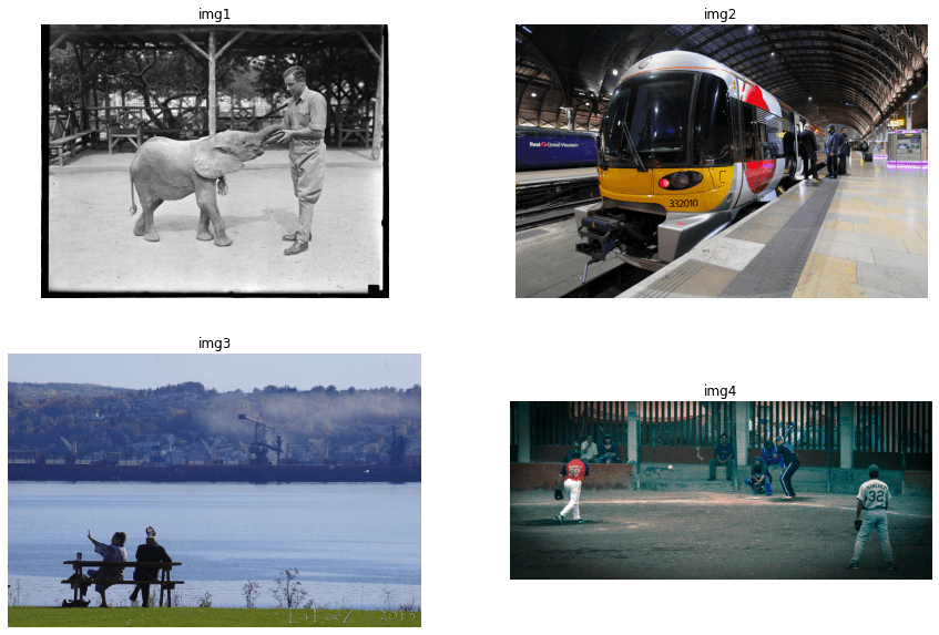
plot_images(image_list, row=2, column=2, fig_size=(15, 10))
COCO Classes
TensorFlow models are trained on the COCO dataset. So we need the class name for the class id map.
category_index = {1: 'person', 2: 'bicycle', 3: 'car', 4: 'motorcycle',
                  5: 'airplane', 6: 'bus', 7: 'train', 8: 'truck', 9: 'boat',
                  10: 'traffic light', 11: 'fire hydrant', 13: 'stop sign',
                  14: 'parking meter', 15: 'bench', 16: 'bird', 17: 'cat',
                  18: 'dog', 19: 'horse', 20: 'sheep', 21: 'cow',
                  22: 'elephant', 23: 'bear', 24: 'zebra', 25: 'giraffe',
                  27: 'backpack', 28: 'umbrella', 31: 'handbag', 32: 'tie',
                  33: 'suitcase', 34: 'frisbee', 35: 'skis', 36: 'snowboard',
                  37: 'sports ball', 38: 'kite', 39: 'baseball bat',
                  40: 'baseball glove', 41: 'skateboard', 42: 'surfboard',
                  43: 'tennis racket', 44: 'bottle', 46: 'wine glass',
                  47: 'cup', 48: 'fork', 49: 'knife', 50: 'spoon', 51: 'bowl',
                  52: 'banana',  53: 'apple',  54: 'sandwich',  55: 'orange',
                  56: 'broccoli',  57: 'carrot',  58: 'hot dog',  59: 'pizza',
                  60: 'donut', 61: 'cake', 62: 'chair', 63: 'couch',
                  64: 'potted plant', 65: 'bed', 67: 'dining table',
                  70: 'toilet', 72: 'tv', 73: 'laptop', 74: 'mouse',
                  75: 'remote', 76: 'keyboard', 77: 'cell phone',
                  78: 'microwave', 79: 'oven', 80: 'toaster', 81: 'sink',
                  82: 'refrigerator', 84: 'book', 85: 'clock', 86: 'vase',
                  87: 'scissors', 88: 'teddy bear', 89: 'hair drier',
                  90: 'toothbrush'}
Class IDs to Color IDs
Let us create color IDs for each class so we can use them to plot bounding boxes of different classes with different colors.
R = np.array(np.arange(0, 256, 63))
G = np.roll(R, 2)
B = np.roll(R, 4)

COLOR_IDS = np.array(np.meshgrid(R, G, B)).T.reshape(-1, 3)
Load Model from TF Hub
To load the model from TF Hub, use the following code.
# ResNet101.
resnet = hub.load(models['Resnet101'])
# Hourglass104.
hourglass = hub.load(models['HourGlass104'])
Run Inference
An inference outcome is a dictionary with the following keys:
- Number of detections
- Detection boxes
- Detection scores
- Detection classes
Let’s make an inference.
# Hourglass104 inference.
result_hourglass = hourglass(np.array([img1]))
Let’s print the keys of the predicted dictionary.
result_hourglass.keys()
dict_keys(['detection_classes', 'detection_scores', 'num_detections', 'detection_boxes'])Let’s check the shapes of the prediction.
print('num_detections shape\t:{}'.format(result_hourglass['num_detections'].shape))
print('detection_boxes shape\t:{}'.format(result_hourglass['detection_boxes'].shape))
print('detection_scores shape\t:{}'.format(result_hourglass['detection_scores'].shape))
print('detection_classes shape\t:{}'.format(result_hourglass['detection_classes'].shape))
num_detections shape	:(1,)
detection_boxes shape	:(1, 100, 4)
detection_scores shape	:(1, 100)
detection_classes shape	:(1, 100)
You can see that the total number of bounding boxes is 100.
Function to Convert Tensors to Numpy
Let’s write a function to convert the TF tensor to NumPy. The function takes the model prediction and returns boxes, scores, and classes.
def to_numpy(prediction):
    result = dict()
    bboxes = prediction['detection_boxes'][0].numpy()
    scores = prediction['detection_scores'][0].numpy()
    # class ids are int
    classes = prediction['detection_classes'][0].numpy().astype(int)
    return bboxes, scores, classes
print_count = 5
bboxes, scores, classes = to_numpy(result_hourglass)
print('detection_boxes:\n{}'.format(bboxes[:print_count]))
print('detection_scores:\n{}'.format(scores[:print_count]))
print('detection_classes:\n{}'.format(classes[:print_count]))
detection_boxes:
[[0.36475214 0.2544147  0.8116531  0.7097043 ]
 [0.15214191 0.6827493  0.84660524 0.82337785]
 [0.30334035 0.85521215 0.4586329  0.94833416]
 [0.36117637 0.19265035 0.48011312 0.2846129 ]
 [0.390655   0.6316224  0.4466164  0.7015844 ]]
detection_scores:
[0.95722336 0.9190534  0.575393   0.48818225 0.46633196]
detection_classes:
[22  1 62 15 44]
Function to Filter Confident Predictions
def filter_detections_on_score(boxes, scores, classes, score_thresh=0.3):
    ids = np.where(scores >= score_thresh)
    return boxes[ids], scores[ids], classes[ids]
score_thresh = 0.30
bboxes, scores, classes = filter_detections_on_score(bboxes, scores, classes,
                                                    score_thresh)
print('detection_boxes:\n{}'.format(bboxes))
print('detection_scores:\n{}'.format(scores))
print('detection_classes:\n{}'.format(classes))
detection_boxes:
[[0.36475214 0.2544147  0.8116531  0.7097043 ]
 [0.15214191 0.6827493  0.84660524 0.82337785]
 [0.30334035 0.85521215 0.4586329  0.94833416]
 [0.36117637 0.19265035 0.48011312 0.2846129 ]
 [0.390655   0.6316224  0.4466164  0.7015844 ]
 [0.3120035  0.02235281 0.52857524 0.1586653 ]
 [0.3826255  0.02449112 0.49790186 0.15688817]
 [0.2699546  0.7290414  0.30082417 0.75153786]]
detection_scores:
[0.95722336 0.9190534  0.575393   0.48818225 0.46633196 0.36656532
 0.36645815 0.31047532]
detection_classes:
[22  1 62 15 44 15 15 32]
Function to Convert Normalized Outputs to Pixel
You can see that the bounding box coordinates are in normalized form. So let’s write a function to convert it into pixel form.
def normalize_to_pixels_bboxs(bboxes, img):
    img_height, img_width, _ = img.shape
    bboxes[:, 0] *= img_height
    bboxes[:, 1] *= img_width
    bboxes[:, 2] *= img_height
    bboxes[:, 3] *= img_width
    return bboxes.astype(int)
bboxes = normalize_to_pixels_bboxs(bboxes, img1)
print('detection_boxes:\n{}'.format(bboxes))
detection_boxes:
[[184 162 409 454]
 [ 76 436 427 526]
 [153 547 231 606]
 [182 123 242 182]
 [197 404 225 449]
 [157  14 266 101]
 [193  15 251 100]
 [136 466 151 480]]
Function to Annotate Detections
def add_prediction_to_image(img, bboxes, scores, classes, id_class_map=category_index, colors=COLOR_IDS):
    img_with_bbox = img.copy()
    for box, score, cls in zip(bboxes, scores, classes):
        top, left, bottom, right = box
        class_name = id_class_map[cls]

        # Bounding box annotations.
        color = tuple(colors[cls % len(COLOR_IDS)].tolist())[::-1]
        img_with_bbox = cv2.rectangle(img_with_bbox, (left, top), (right, bottom), color, thickness=2)
        display_txt = '{}: {:.2f}'.format(class_name, score)
        ((text_width, text_height), _) = cv2.getTextSize(display_txt, cv2.FONT_HERSHEY_SIMPLEX, 1.0, 2)
        img_with_bbox = cv2.rectangle(img_with_bbox, (left, top - int(0.9 * text_height)), (left + int(0.4*text_width), top), color, thickness=-1)
        img_with_bbox = cv2.putText(img_with_bbox, display_txt, (left, top - int(0.3 * text_height)), cv2.FONT_HERSHEY_SIMPLEX, 0.4, (0, 0, 0), 1)

    return img_with_bbox
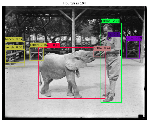
annotated_img = add_prediction_to_image(img1, bboxes, scores, classes)
plot_images([annotated_img], ['Hourglass 104'],row=1, column=1, fig_size=(10, 10))
Wrap-Up Inference, Annotation, and Plotting
It’s time to put everything together.
The following function accepts an image, the model, and a score threshold. The image is forward passed to get all the bounding box predictions. These are further filtered by the function filter_detection_on_score and annotated by the function add_prediction_to_image. This function returns the image with predictions annotated.
def infer_and_add_prediction_to_image(img, model, score_thresh=0.3):
    prediction = model(np.array([img]))
    bboxes, scores, classes = to_numpy(prediction)

    bboxes, scores, classes = filter_detections_on_score(bboxes, scores, classes,
                                                        score_thresh)
    boxes = normalize_to_pixels_bboxs(bboxes, img)
    img_with_bboxes = add_prediction_to_image(img, boxes, scores, classes)
    return img_with_bboxes
Let’s use the above function with img1 and the ResNet model.
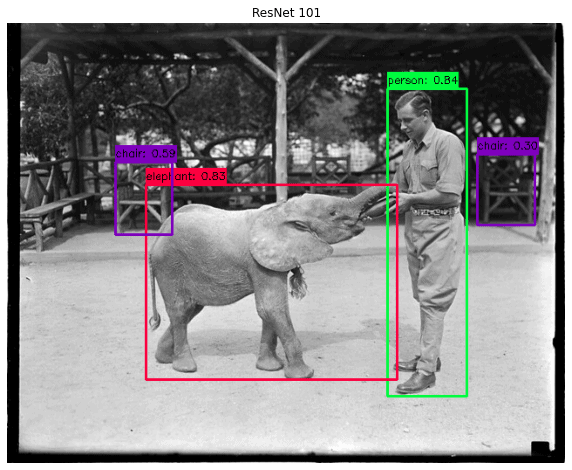
annotated_img = infer_and_add_prediction_to_image(img1, resnet)
plot_images([annotated_img], ['ResNet 101'], row=1, column=1, fig_size=(10, 10))
Let’s write a wrapper function that takes an image, makes inferences on both Hourglass and ResNet models, and plots filtered detection.
def show_hourglass_resnet_inference(img, score_thresh=0.3):
    hourglass_infer = infer_and_add_prediction_to_image(img, hourglass)
    resnet_infer = infer_and_add_prediction_to_image(img, resnet)
    image_list = [hourglass_infer, resnet_infer]
    titles = ['Hourglass 104', 'ResNet 101']
    plot_images(image_list, titles, row=1, column=2, fig_size=(20, 10))
Results
Let’s use the above function for all four images one by one.
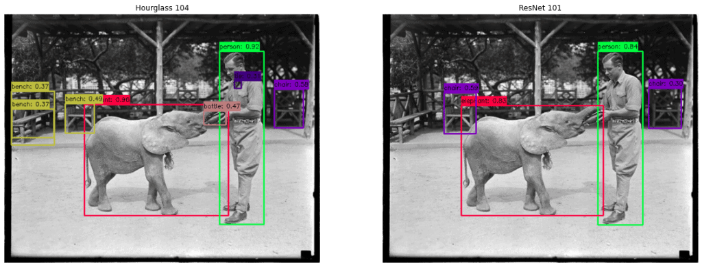
show_hourglass_resnet_inference(img1)
show_hourglass_resnet_inference(img2)

show_hourglass_resnet_inference(img3)

show_hourglass_resnet_inference(img4)

Here, you can notice that Hourglass 104 model is better than ResNet 101.
Conclusion
- CenterNet Object as Points is an anchor free object detector. Because of its generalizability, it can be used for human pose estimation, 3D detection, and much more.
- It uses heatmaps to select the predicted object that removes the requirements of NMS.
- TensorFlow hub has pre-trained CenterNet models with Hourglass, ResNet, and DLA backbone that can be used for inference and finetuning.
Must Read
- YOLOX Object Detector Paper Explanation and Custom Training
- YOLOv6 Object Detection – Paper Explanation and Inference
- YOLOv7 Object Detection Paper Explanation and Inference
- Fine Tuning YOLOv7 on Custom Dataset
- Multiple Object Tracking using FairMOT (based on CenterNet)
References
- https://arxiv.org/abs/1904.07850
- https://arxiv.org/abs/1904.08189
- https://arxiv.org/abs/1612.03144
- https://arxiv.org/abs/1708.02002
- https://arxiv.org/abs/1808.01244
- https://github.com/xingyizhou/CenterNet
- https://tfhub.dev/tensorflow/collections/object_detection/1




100K+ Learners
Join Free OpenCV Bootcamp3 Hours of Learning