OpenCV feature matching techniques are some powerful algorithms. They are useful in many cases, even today in 2025. In this blogpost, you will learn OpenCV Feature Matching by building a fun game player bot. Do you think you will be able to beat my highest score? Continue reading to find out more.
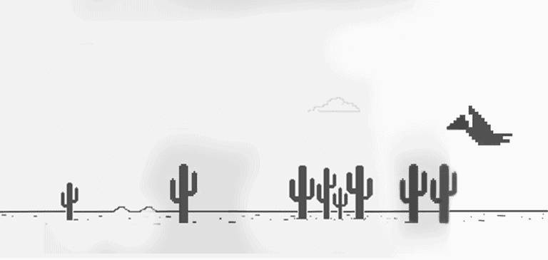
Chrome Dino Bot Application Planning
To make the bot that will control the game externally, we need a way to capture the screen and process the frames in real-time to detect the player (T-rex) position on the screen and trigger keypress automatically when an obstacle is about to hit it.
We will use the mss library to capture the scene. We can simply perform contour analysis on an area in front of the player to detect an obstacle. To simulate keypress, we can use AutoPyGUI. But how do we obtain the area? You may suggest training a TensorFlow or Caffe model and using the OpenCV DNN module to detect the player position. That’s not a bad idea, but with the ever-increasing hype in ML, we forget about some fantastic classic tools available in OpenCV.
Feature Matching is a powerful technique that can detect specific objects based on just one reference image.
1. What is Feature Matching in Computer Vision?
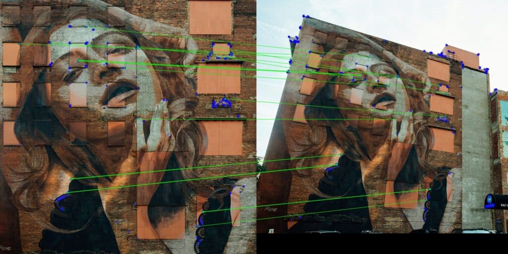
Feature Matching in computer vision consists of three parts.
- Feature Detector or Keypoint Detector: Certain features in an image are easy to detect and locate. Typically, we want features to be corner-like to precisely locate them in two different images of the same scene. A feature detector provides x and y coordinates of the feature in the images. Harris corner detector is an example of a feature detector.
- Feature Descriptor: Given the location of the feature detected using a Feature Detector, the job of the Feature Descriptor is to define a “signature” for the feature to match the feature across two or more images of the same scene. The input to a Feature Descriptor is the location (x, y) in the image, and the output is a vector of numbers (signature). A good Feature Descriptor will create similar vectors for the same feature in two or more different images. FREAK is an example of a Feature Descriptor. On the other hand, SIFT, SURF, and ORB contain a combination of a Feature Detector and a Feature Descriptor.
- Feature Matching Algorithm: To identify an object in two different images, we identify features in the two images and match them using a Feature Matching algorithm. A Brute Force Algorithm is employed when the number of images over which we need to do feature matching is small. However, if we need to search an image in a large database of images, we have to use FLANN (Fast Library for Approximate Nearest Neighbors.)
SIFT, SURF, and ORB
Let’s look at some Feature Detector + Descriptors.
David G. Lowe invented Scale Invariant Feature Transform or SIFT in 2004. It had a huge impact on computer vision, and until the advent of Deep Learning, SIFT was the dominant handcrafted feature. It is based on the DoG (Difference of Gaussian Detector).
We want the Feature Descriptor to remain the same when the image undergoes certain geometrical transformations. In other words, we want the descriptor to be invariant to such geometric transformations as scale, translation, rotation, translation, and affine transformation.

SIFT was a good descriptor invariant to the above transformations, but it was slow and was patented by the University of British Columbia. So you had to pay to use SIFT.
Fun fact: The SIFT patent expired in March 2020, and the good folks at OpenCV moved the algorithm from opencv-contrib to the main OpenCV repository.
SURF stands for Speed Up Robust Features. Released in 2006. It is faster than SIFT but again it has the disadvantage of being patented. You need to compile OpenCV from scratch, enabling a certain flag to use these algorithms, i.e., OPENCV_ENABLE_NONFREE = ON.
ORB, BRISK, and FREAK are faster and most importantly, not patent-encumbered. BEBLID (Boosted Efficient Binary Local Image Descriptor) is another improved algorithm, released recently with OpenCV 4.5.1.
Now, let’s understand how ORB (Oriented FAST and Rotated BRIEF) detects and computes features. Invented by Ethan Rublee, ORB was released in 2011. It uses FAST (Features from Accelerated Segment Test) to detect features and to compute descriptors it uses BRIEF (Binary Robust Independent Elementary Features). It’s been 11 years and ORB still stands strong. Recently, the paper received ICCV 2021 Helmholtz Prize for creating such an impact on computer vision research.
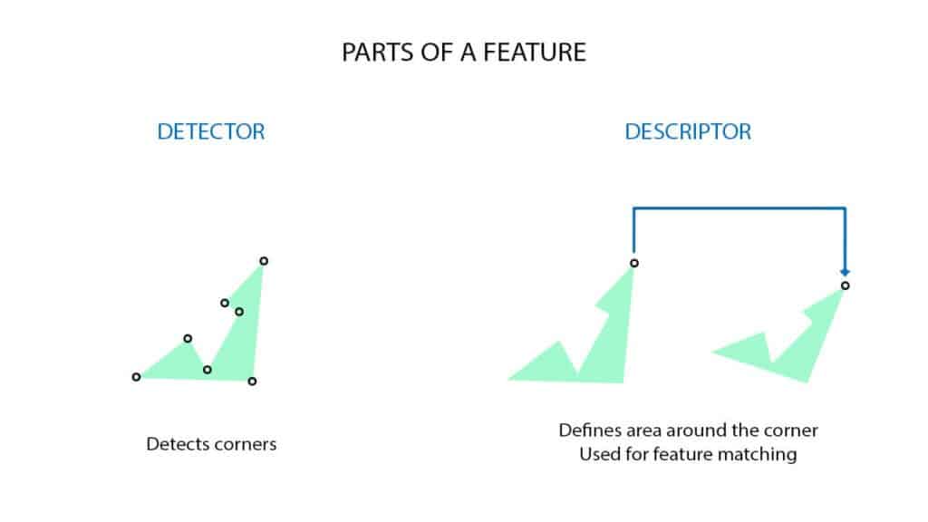
1.1 How does ORB work?
Let us consider the top corner of the shape shown above to understand it’s working. After converting to grayscale, any corner in an image will either have a bright pixel with a darker background or a dark pixel with a brighter background. The FAST algorithm looks at four pixels in the neighborhood and compares the intensities with the center pixels. The following illustration shows the working of the algorithm.
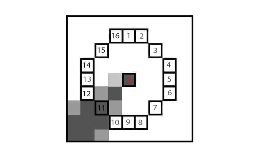
Take an image patch, let Ic be the intensity of the center pixel. Consider 16 pixels around it with intensities I1, I2, …, I16. Select a threshold intensity T. The pixel at the center is marked as a corner if one of the following conditions is met.
- For darker corners: There are n continuous pixels where In > Ic + T.
- For brighter corners: There are n continuous pixels where In < Ic – T.
For most pixels, we can just look at pixels 1, 5, 9, and 13 to determine a corner. If at least 3 out of 4 pixels are darker or brighter than the center pixel then we can declare it as a corner point.
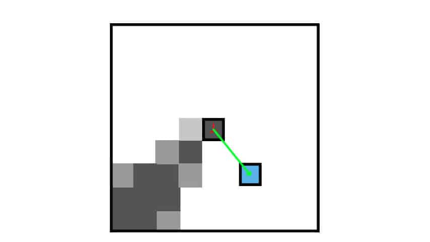
Next, we need to calculate the orientation of the feature. It is done by finding the centroid of the patch. It’s nothing but the orientation of the line joining the center pixel and the centroid, the blue pixel shown in the illustration. It is found using image moments. Curious to know how it is found using OpenCV? Check out this blogpost.
To match the features successfully, we also need a little bit of something, a brief description of the image patch as you may recall. The BRIEF descriptor randomly selects two points at a time, compares the intensities, and constructs a vector that acts as a signature of the patch. The number of times it compares two random pixels is equal to the bit length of the descriptor.
Now, once we have the key points and descriptors, we can use the data and pass it onto a descriptor matcher to find matches. In OpenCV, there are two types of descriptor matchers. BRUTE FORCE based and FLANN based.
1.2 ORB in OpenCV
In OpenCV, there are three main functions: ORB_create(), detect() and compute(). However, it can be further simplified by using the detectAndCompute() function directly.
Function Syntax
- Create an orb object.
orb = cv2.ORB_create(nFeatures,
                        scaleFactor,
                        nlevels,
                        edgeThreshold,
                        firstLevel,
                        WTA_K,
                        scoreType,
                        patchSize,
                        fastThreshold)
Parameters:
- nFeatures is the number of maximum key points that we want.
- scaleFactor is the pyramid decimation ratio. The default value is 1.2. Ranges from 1 – 2.
- nLevels is the number of pyramid levels. The default value is 8.
- edgeThreshold is the size of the border where features are not detected. Default value 31.
- firstLevel is the level of the pyramid to put the source image to. The default value is 0.
- WTA_K is the number of points that produce each element of the oriented brief descriptor. The default value is 2.
- scoreType is the algorithm that is used to rank features. The default value is HARRIS_SCORE. Another available algorithm is FAST_SCORE.
- patchSize is as the name suggests, the size of the image patch used by the oriented brief descriptor. The default value is 31.
- fastThreshold is the threshold intensity used by FAST while detecting feature points. The default threshold intensity is 20.
Except for nFeatures, the rest of the arguments can be kept as default. You may check the official documentation for further information.
- Detect feature
keypoints = orb.detect(image, mask)
- Compute descriptors
keypoints, des = orb.compute(image, keypoints, mask)
- Detect and compute.
keypoints, des = orb.detectAndCompute(image, mask)
To detect and compute features, we can also pass a binary mask that tells the algorithm to work on the required area. Otherwise, None is passed.
1.3 Descriptor Matcher in OpenCV.
As mentioned earlier, in OpenCV there are two types of descriptor matchers, based on two different algorithms, BRUTE FORCE, and FLANN. Just like ORB, here also we need to create a descriptor matcher object and then find matches using match() or knnMatch().
Function Syntax
- Create Descriptor matcher.
retval = cv2.DescriptorMatcher_create(descriptorMatcherType)
Types of descriptor matcher:
i. FLANNBASED
ii. BRUTEFORCE
iii. BRUTEFORCE_L1
iv. BRUTEFORCE_HAMMING
v. BRUTEFORCE_HAMMING_LUT
vi. BRUTEFORCE_SL2
- Match descriptors.
retval = cv2.DescriptorMatcher.match(queryDescriptors, trainDescriptors, mask)
Since feature matching is computationally inexpensive it is extensively used in various interesting applications like document scanner apps, panorama, image alignment, object detection, face detection, etc. With this, let’s go ahead and start building the bot.
2. Chrome Dino Gameplay Observation and Challenges
You can open the game in any browser but it is best optimized for chrome and hence it is recommended. Type chrome://dino in Chrome’s address bar to load the game. In the game, we observe that all the cactus obstacles can be jumped with proper jump timing but for the birds, we may need to duck sometimes depending upon the level of the bird.
The bird appears in three different height levels, high, middle, and low. When it approaches in low height, it can be jumped. For middle height, it can be either jumped or ducked. Spacebar key to jump and down arrow key to duck.
If it appears above head level, nothing needs to be done. The t-rex can simply pass it. The t-rex moves forward a little when the game starts and after that, the position is constant throughout the game. The game mode changes between day and night at some interval.
3. Chrome Dino Bot Application Workflow
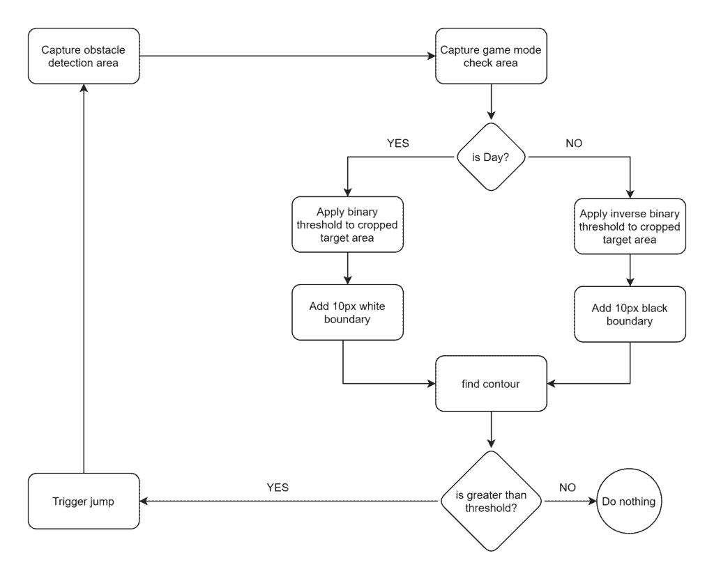
Based on the observations stated above, the application workflow has been designed as follows.
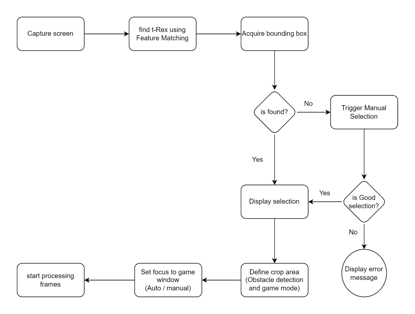
3.1 Chrome Dino Bot Application Processing Loop
3.2 PREREQUISITES
We are going to use opencv-python, mss, and pyautogui for the above-mentioned tasks. Use the requirements.txt file provided within the codes directory to install all necessary packages. Assuming that you already have python and pip installed in your system, you can open terminal or PowerShell, navigate to the downloaded code directory and enter the following command.
pip install -r requirements.txt
3.3 BOT IN ACTION
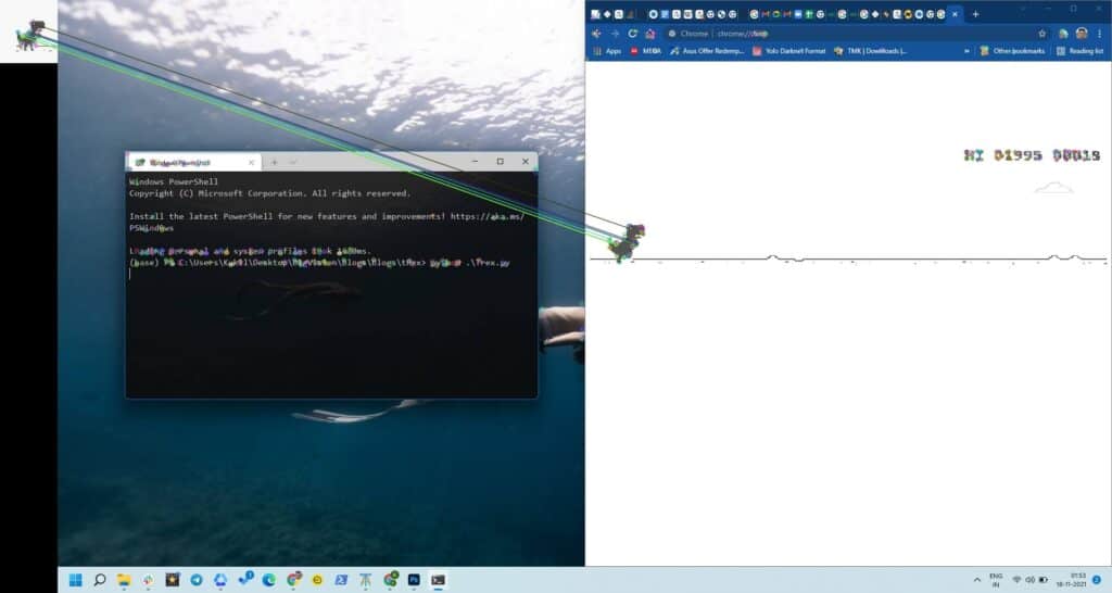
Fig. 3.3.1 Finding matches using a reference t-rex image.

Fig. 3.3.2 Displaying obstacle detection area.
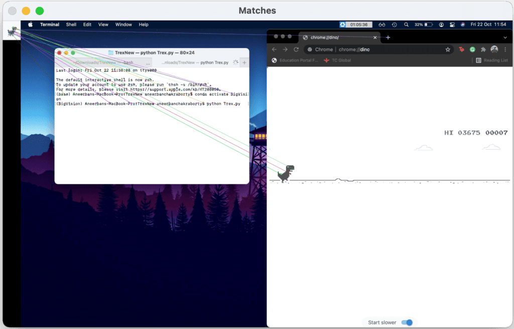
Fig. 3.3.3 Possible fail case due to the presence of black text and white background terminal on the left side.
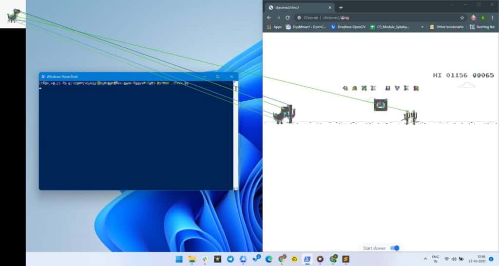
Fig. 3.3.4 Another possible fail case.

3.3.5 Redundancy function triggering.
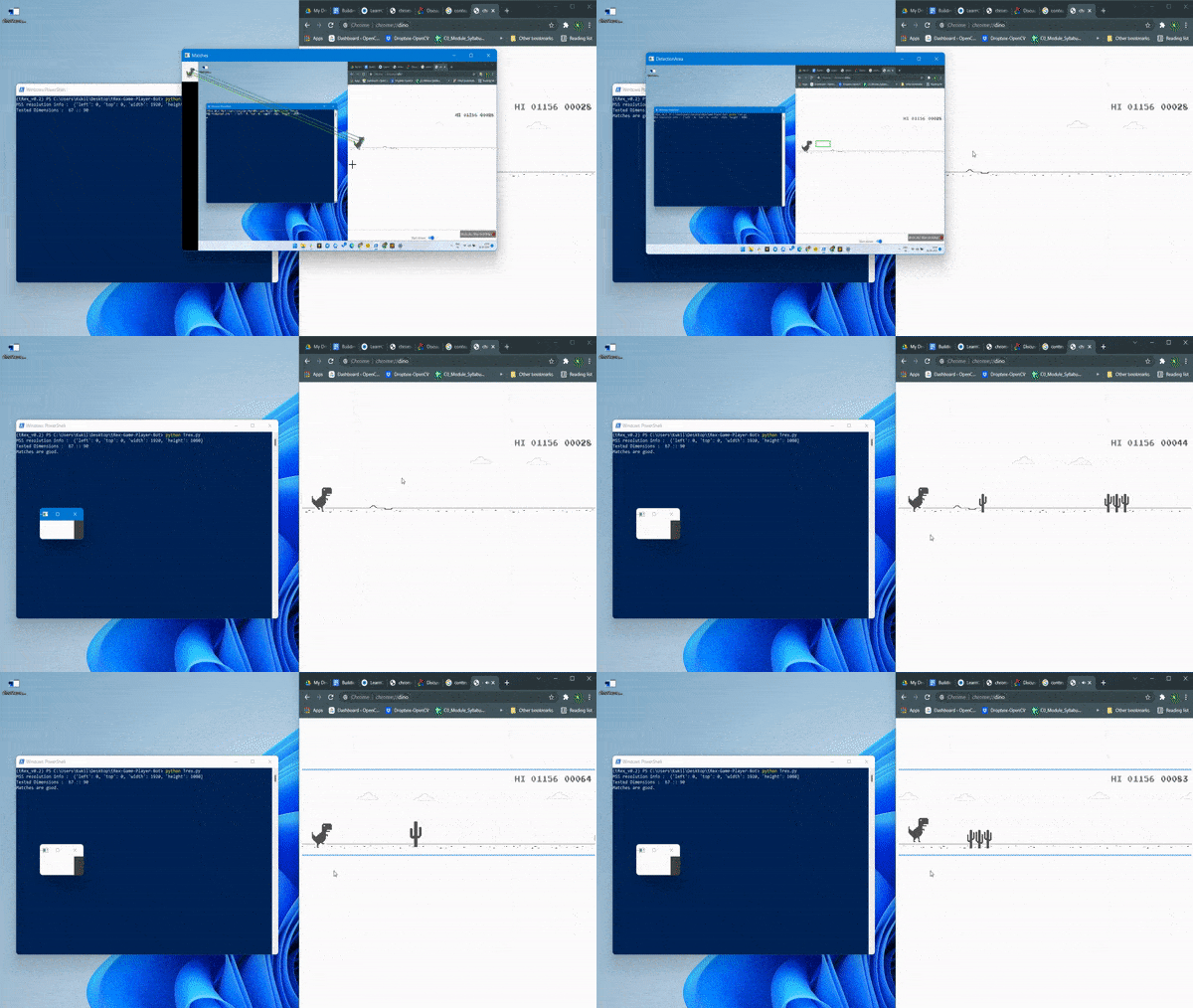
3.3.6 Bot working GIF
5. Chrome Dino Bot Code Explanation
Before executing the code, I will suggest you go through the code once. Read the explanation thoroughly as you might need to change a few parameters based on your system. Jump to the execution part.
5.1 Imports
Let’s import the necessary libraries. Apart from usual packages, mss is used for screen capture, Tkinter is used for showing error messages and pyautogui does the job for a virtual keypress.
import cv2
import numpy as np
# MSS library for screen capture.
from mss import mss
from tkinter import *
# PyAutoGUI for controlling keyboard inputs.
import pyautogui as gui
# Message box to show error message prompt.
import tkinter.messagebox
5.2 Function to detect the t-rex.
Based on the reference image (Ground Truth) of the t-rex that we have, we find the t-rex on the screen using feature matching. The functions take the ground truth image and captured screen image as arguments. As shown below, ORB has been used to detect and compute the key points and descriptors of both images. Then we use a descriptor matcher to find the matches. At last, matches are sorted and filtered. The top 25% of them are taken as good matches. You can play with this value to generate optimum results.
The function returns the key points as a list, which will be used later to estimate the t-rex position.
def getMatches(ref_trex, captured_screen):
    # Initialize lists
    list_kpts = []
    # Initialize ORB.
    orb = cv2.ORB_create(nfeatures=500)
    # Detect and Compute.
    kp1, des1 = orb.detectAndCompute(ref_trex, None)
    kp2, des2 = orb.detectAndCompute(captured_screen, None)
    # Match features.
    matcher = cv2.DescriptorMatcher_create(cv2.DESCRIPTOR_MATCHER_BRUTEFORCE_HAMMING)
    matches = matcher.match(des1, des2, None)
    # Convert to list.
    matches = list(matches)
    # Sort matches by score.
    matches.sort(key=lambda x: x.distance, reverse=False)
    # Retain only the top 25% of matches.
    numGoodMatches = int(len(matches) * 0.25)
    matches = matches[:numGoodMatches]
    # Visualize matches.
    match_img = cv2.drawMatches(ref_trex, kp1, captured_screen, kp2, matches[:50], None)
    # For each match...
    for mat in matches:
        # Get the matching keypoints for each of the images.
        img2_idx = mat.trainIdx
        # Get the coordinates.
        (x2, y2) = kp2[img2_idx].pt
        # Append to each list.
        list_kpts.append((int(x2), int(y2)))
    # Resize the image for display convenience.
    cv2.imshow('Matches', cv2.resize(match_img, None, fx=0.5, fy=0.5))
    # cv2.imwrite('Matches.jpg', match_img)
    cv2.waitKey(0)
    cv2.destroyAllWindows()
    return list_kpts
5.3 Redundancy function
This is a mouse callback function, triggered when feature matching fails. Adding click-drag-release functionality to define the obstacle detection patch coordinates. This is the area where we perform contour analysis to check if there is any obstacle in it. When the left button is pressed, the coordinates of that point are stored in the top_left_corner list and upon releasing the left mouse button, the coordinates are stored in the botton_right_corner list. The rectangle is drawn on the frame once the left mouse button is released.
This area determines the success of the bot. Feel free to try out different regions in front of the t-rex.
def drawBboxManual(action, x, y, flags, *userdata):
    global bbox_top_left, bbox_bottom_right
    # Text origin coordinates estimated on the right half using following logic.
    '''
    Divide the screen into 12 columns and 3 rows. The origin of the text is defined at
    3rd row, 6th column.
    '''
    org_x = int(6 * img.shape[1] / 12)
    org_y =  int(3 * img.shape[0] / 5)

    # Display Error Text.
    cv2.putText(img, 'Error detecting Trex', (org_x + 20, org_y - 20),
                cv2.FONT_HERSHEY_SIMPLEX, 0.65, (0, 0, 255), 1, cv2.LINE_AA)
    cv2.putText(img, 'Please click and drag', (org_x + 20, org_y),
                cv2.FONT_HERSHEY_SIMPLEX, 0.65, (0, 0, 255), 1, cv2.LINE_AA)
    cv2.putText(img, 'To define the target area', (org_x + 20, org_y + 30),
                cv2.FONT_HERSHEY_SIMPLEX, 0.65, (0, 0, 255), 1, cv2.LINE_AA)
    # Mouse interactions.
    if action == cv2.EVENT_LBUTTONDOWN:
        # Acquire the coordinates (stored as a list).
        bbox_top_left = [(x, y)]
        # center_1 : centre of point circle to be drawn.
        center_1 = (bbox_top_left[0][0], bbox_top_left[0][1])
        # Draw a small filled circle.
        cv2.circle(img, center_1, 3, (0, 0, 255), -1)
        cv2.imshow("DetectionArea", img)

    if action == cv2.EVENT_LBUTTONUP:
        # Acquire the coordinates (stored as a list).
        bbox_bottom_right = [(x, y)]
        # center_1 : centre of point circle to be drawn.
        center_2 = (bbox_bottom_right[0][0], bbox_bottom_right[0][1])
        # Draw a small filled circle.
        cv2.circle(img, center_2, 3, (0, 0, 255), -1)
        # Define top left corner and bottom right corner coordinates of the bounding box as tuples.
        point_1 = (bbox_top_left[0][0], bbox_top_left[0][1])
        point_2 = (bbox_bottom_right[0][0], bbox_bottom_right[0][1])
        # Draw bounding box.
        cv2.rectangle(img, point_1, point_2, (0, 255, 0), 2)
        cv2.imshow("DetectionArea", img)
    cv2.imshow("DetectionArea", img)
    # cv2.imwrite('MouseDefinedBox.jpg', cv2.resize(img, None, fx=2, fy=2, interpolation=cv2.INTER_AREA))
5.4 Check day or night function
We are taking a region just above the obstacle detection patch, and checking whether the game mode is day or night. The logic is very simple, for night mode, as the image is black; maximum pixels in the image will have intensities close to zero. On the other hand for day mode, maximum pixels will have intensities closer to 255.
Here, the function returns the average intensity value. This value will be used later in condition statements to make sure that contour analysis works in either of the cases.
def checkDayOrNight(img):
    # List to hold pixel intensities of a patch.
    pixels_intensities = []
    img = cv2.cvtColor(img, cv2.COLOR_BGR2GRAY)
    h = int(img.shape[0] / 4)
    w = int(img.shape[1] / 4)
    for i in range(h):
        for j in range(w):
            pixels_intensities.append(img[i, j])
    # Find average pixel intensities.
    val = int(sum(pixels_intensities) / len(pixels_intensities))
    # If greater than 195, consider day mode.
    if val > 195:
        return True
    else:
        return False
5.5 Initializations
Here we set pyautogui keypress delay to 0ms so that the loop runs smoothly in real-time.
# Set keypress delay to 0.
gui.PAUSE = 0

# Initialize lists to hold bounding box coordinates.
bbox_top_left = []
bbox_bottom_right = []
5.6 MAIN FUNCTION
5.6.1 Load ground truth and capture screen.
The downloaded code file contains two reference images. One for normal mode and the other for dark mode. Make sure to comment and uncomment the lines based on your system mode. You can also take a screenshot of your screen and crop out the reference image if you want.
Next, we capture the screen using mss screengrab. screen.monitors[1] returns a dictionary that contains the top, left, width, and height of the display. In my case (no external display attached), it returns the same value for both monitors[0] and monitors[1]. Make sure to check the output for multi-display setups and especially if you are using a MacBook as it has an auto-scaling feature.
 # Load reference image.
 ref_img = cv2.imread('trex.png')
 # Uncomment the following line if you are on Dark Mode.
 # ref_img = cv2.imread('tRexDark.jpg')
 screen = mss()
 # Identify the display to capture.
 monitor = screen.monitors[1]
 # Check resolution info returned by mss.
 print('MSS resolution info : ', monitor)
 # Grab the screen.
 screenshot = screen.grab(monitor)
 # Convert to numpy array.
 screen_img = np.array(screenshot)
Note that we need to convert the captured data to a numpy array before passing it to cv2 operations.
5.6.3 Analyze t-rex dimension with respect to the screen resolution.
It’s based on the assumption that we position the chrome window covering approximately half of the screen as shown in the figures above. We have tested it on full HD and 4k display and obtained the approximate size of the t-rex according to the resolution.
You might want to test the ratio once if your system has a different resolution. Just capture the screen, crop the t-rex, obtain dimensions and divide it by system resolution.
 # Define Tested height and width of TRex, according to the screen resolution.
    box_h_factor = 0.062962
    box_w_factor = 0.046875
    hTrex = int(box_h_factor * screen_img.shape[0])
    wTrex = int(box_w_factor * screen_img.shape[1])
    tested_area = hTrex * wTrex
    # print('Tested Dimensions : ', hTrex, '::', wTrex)
5.6.4 Find matches
Using the function getMatches() we acquire the key points of the t-rex which are returned by the function as a list. Hence, it has to be converted to an array before passing into the boundingRect() function which returns the bounding box dimensions estimated from the array. Now that we have the bounding box of the t-rex, it can be compared with the tested dimensions and decide whether it is a good detection or not.
# Obtain key points.
trex_keypoints = getMatches(ref_img, screen_img)
# Convert to numpy array.
kp_arary = np.array(trex_keypoints)
# Get dimensions of the bounding rectangle.
x, y, w, h = cv2.boundingRect(np.int32(kp_arary))
obtained_area = w * h
5.6.5 Estimate obstacle detection region
From a set of tests, we observed that if the obtained bounding box area is in the range of 10% to 300% of the tested area, it’s a good detection. The obstacle detection region is set to occupy the front area of the t- rex by shifting the bounding box to the right.
You can play with the shift amount to check what works best. If the detection fails to satisfy the area condition, we trigger the redundancy function that asks you to draw the bounding box using the mouse or touchpad in front of the t-rex.
 if 0.1*tested_area < obtained_area < 3*tested_area:
        print('Matches are good.')
        # Set Target area bbox coordinates.
        xRoi1 = x + wTrex
        yRoi1 = y
        xRoi2 = x + 2 * wTrex
        """
        Set the height of the bbox at 50% of the original. To make sure  that it does not capture the line below the T-Rex. You can play with this value to come up with better positioning.
        """
        yRoi2 = y + int(0.5*hTrex)
        # Draw a rectangle.
        cv2.rectangle(screen_img, (xRoi1, yRoi1), (xRoi2, yRoi2), (0, 255, 0), 2)
        cv2.imshow('DetectionArea', cv2.resize(screen_img, None, fx=0.5, fy=0.5))
        cv2.imwrite('ScreenBox.jpg', screen_img)
        cv2.waitKey(0)
        cv2.destroyAllWindows()

    else:
        print('Matches are not good, please set target area manually.')
        img = cv2.resize(screen_img, None, fx=0.5, fy=0.5)
        cv2.namedWindow('DetectionArea')
        cv2.setMouseCallback('DetectionArea', drawBboxManual)
        cv2.imshow('DetectionArea', img)
        cv2.waitKey(0)
        cv2.destroyAllWindows()
        # Resize back and set Target area bbox coordinates accordingly.
        xRoi1 = 2 * bbox_top_left[0][0]
        yRoi1 = 2 * bbox_top_left[0][1]
        xRoi2 = 2 * bbox_bottom_right[0][0]
        yRoi2 = 2 * bbox_bottom_right[0][1]
5.6.6 Halt the program if the bounding box is not drawn properly.
This is to counter screen capture errors raised by wrong input. Usually occurs with a touchpad. Where click-drag-click occurs instead of click-drag-lift. We are using Tkinter to generate the error message when this occurs.
    # If you click-drag performed wrong, restart.
    if xRoi1 == xRoi2 and yRoi1 == yRoi2:
        print('Please draw the bounding box again using click-drag-release method not click-drag-click')
        window = Tk()
        window.wm_withdraw()
        # Error message at the center of the screen.
        win_width = str(window.winfo_screenwidth()//2)
        win_height = str(window.winfo_screenheight()//2)
        window.geometry("1x1+"+win_width+"+"+win_width)
        tkinter.messagebox.showinfo(title="Error", message="Please use click-drag-release")
        exit()
5.6.7 Adjust scaling and define screen capture dictionary.
MSS library requires a dictionary to capture screens. Here, scaling adjustment is required only if the screen resolution returned by mss is different from the actual screen resolution.
You can check it by printing the mss.monitors[1]. It returns a dictionary containing the screen width and height. The factor can be obtained by dividing the dimension returned by mss with the actual resolution. With this, we define the dictionaries for obstacle detection and game mode determining regions.
# xRoi1, yRoi1, xRoi2, yRoi2 = (xRoi1 // 2, yRoi1 // 2, xRoi2 // 2, yRoi2 // 2)

# Create a dictionary for MSS, defining the size of the screen to be captured.
obstacle_check_bbox = {'top': yRoi1, 'left': xRoi1, 'width': xRoi2 - xRoi1, 'height': yRoi2 - yRoi1}
# Day or Night mode checking patch. Estimated just above obstacle detecting patch.
day_check_bbox    = {'top': yRoi1 - 2*hTrex, 'left': xRoi1, 'width': xRoi2, 'height': yRoi2 - 2*hTrex}
5.7 Main Loop
With the dictionaries defined above, we capture the screen. So at every instant, two image patches are being captured. The first is the obstacle detection patch and the second is the game mode checking region.
The function checkDayOrNight returns a boolean based on the game mode. When the environment is bright (Day mode) it returns True. This check is necessary because for day mode, the environment is white and voids are black.
TRESH_BINARY works best in day mode but as the mode changes to night, the environment is black and voids are white. Here we need to change the mode to THRESH_BINARY_INV otherwise findContours function will not work.
We are also using the copyMakeBorder function to create a 10px boundary so that findContours works even if the obstacle is touching the boundary. As you can see, the borders are made black for daytime and white for nighttime.
The rest is just contour analysis, where we trigger the space bar key using pyautogui. Triggered when the number of contours is more than one.
while True:
    # Capture obstacle detecting patch.
    obstacle_check_patch = screen.grab(obstacle_check_bbox)
    obstacle_check_patch = np.array(obstacle_check_patch)

    # Day or Night mode checking patch.
    day_check_patch = screen.grab(day_check_bbox)
    day_check_patch = np.array(day_check_patch)

    # Convert obstacle detecting area to grayscale.
    obstacle_check_gray = cv2.cvtColor(obstacle_check_patch, cv2.COLOR_BGR2GRAY)

    # Check the game mode.
    day = checkDayOrNight(day_check_patch)

    # Perform contour analysis according to the game mode.
    if day:
        # Add 10px padding for effective contour analysis.
        obstacle_check_gray = cv2.copyMakeBorder(obstacle_check_gray, 10, 10, 10, 10,
                                         cv2.BORDER_CONSTANT, None, value=255)
        # Perform thresholding.
        ret, thresh = cv2.threshold(obstacle_check_gray, 127, 255,
                                    cv2.THRESH_BINARY)
    else:
        # Add 10px padding for effective contour analysis.
        obstacle_check_gray = cv2.copyMakeBorder(obstacle_check_gray, 10, 10, 10, 10,
                                         cv2.BORDER_CONSTANT, None, value=0)
        # Perform thresholding.
        ret, thresh = cv2.threshold(obstacle_check_gray, 127, 255,
                                    cv2.THRESH_BINARY_INV)

    # Find contours.
    contours, hierarchy = cv2.findContours(thresh, cv2.RETR_LIST,
                                           cv2.CHAIN_APPROX_NONE)
    # Print number of contours.
    # print('Contours Detected : ', len(contours))

    # Make the T-Rex jump.
    if len(contours) > 1:
        gui.press('space', interval=0.1)

    cv2.imshow('Window', obstacle_check_gray)
    key = cv2.waitKey(1)
    if key == ord('q'):
        cv2.destroyAllWindows()
        break
Chrome Dino Bot Execution
As suggested before, position your chrome window to the right half of the screen. Make sure to minimize other windows if present. Open terminal / PowerShell on the left free space. Do not let it overlap the chrome window. Go to chrome://dino and start the game.
You will notice the game adjusts the scale to match the resized chrome window. It’s important to start the game as the t-rex moves forward a little at the start. Once it begins, there is no pause button, hence you’ll have to click anywhere outside chrome to pause it.
When you have the setup ready, something like shown above, you can run the script. Don’t forget to click on the chrome window after you run it.
Chrome Dino Bot Possible Fail Cases
As shown before, the following situations may lead to inefficient feature matching.
- Using white background reference image while in dark mode or the other way.
- If the terminal color is similar ( Black and white), text corners may get detected as the t-rex.
- Setting a higher percentage of features as good features.
- Scaling adjustment done wrong.
All the issues can be tackled easily. If required, go through the explanation once again.
CONCLUSION
So that’s all for the T-Rex Game Bot using OpenCV feature matching. We have to agree to the fact that it’s not perfect but if we compare it to deep learning-based detection techniques, it’s far more efficient and easier to implement. Imagine how much time it would have taken to train a model just to detect the t-rex. Using feature matching, we can solve such issues with a bare minimum of adjustments. I hope this blogpost helped you understand OpenCV Feature Matching and hinted you to some brilliant new ideas on its application.


