


In a previous post, we covered the concept of fully convolutional neural networks (FCN) in PyTorch, where we showed how we could solve the classification task using the input image of arbitrary size.
We received several requests for the same post in Tensorflow (TF). By popular demand, in this post, we implement the concept using TF
TensorFlow Fully Convolutional Neural Network – TensorFlow FCN
Let’s start with a brief recap of what Fully Convolutional Neural Networks are.
Fully connected layers (FC) impose restrictions on the size of model inputs. If you have used classification networks, you probably know that you must resize and/or crop the image to a fixed size (e.g. 224×224).
To feed an arbitrary-sized image into the network, we need to replace all FC layers with convolutional layers, which do not require a fixed input size.
In the previous fully convolutional network implementation, we used a pre-trained PyTorcnnch ResNet-18 network as a baseline for its further modification into a fully convolutional network.
Fully Convolutional ResNet-50
We wanted to replicate the above implementation in TensorFlow. However, ResNet-18 is not available in TensorFlow as tensorflow.keras.applications contain pre-trained ResNet models starting with a 50-layer version of ResNet. That’s why in the current post, we will experiment with ResNet-50.
This network expects an input image of size 224×224×3. Before we start the ResNet-50 transformation into a fully convolutional network, let’s review its architecture.


Each ResNet-50 block is 3-layer deep, whereas ResNet-18 blocks are 2-layer deep.
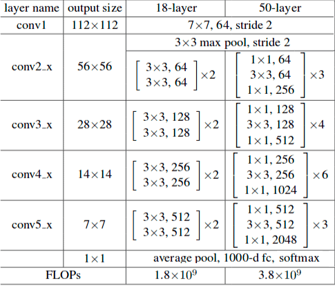
You can see in Figure 1, the first layer in the ResNet-50 architecture is convolutional, which is followed by a pooling layer or MaxPooling2D in the TensorFlow implementation (see the code below). This, in turn, is followed by 4 convolutional blocks containing 3, 4, 6 and 3 convolutional layers.
Finally, we have a global average pooling layer called as GlobalAveragePooling2D in the code. The output of this layer is flattened and fed to the final fully connected layer denoted by Dense. However, there is also another option in TensorFlow ResNet50 implementation regulated by its parameter include_top. When it is set to True, which is the default behaviour, our model keeps the last fully connected layer. If we set this value to False the last fully connected layer will be excluded. Another parameter such as pooling, can be used in case, when include_top is set to False. If pooling is None the model will return the output from the last convolutional block, if it is avg then global average pooling will be applied to the output, and if it is set to max – global max pooling will be used instead.
The below code was snipped from the resnet50.py file – the ResNet-50 realization in TensorFlow adapted from tf.keras.applications.ResNet50. You can compare its architecture with the table above.

# ResNet50 initial function
def ResNet50(include_top=True,
             weights='imagenet',
             input_tensor=None,
             input_shape=None,
             pooling=None,
             classes=1000,
             **kwargs):
  """Instantiates the ResNet50 architecture."""

  def stack_fn(x):
    x = stack1(x, 64, 3, stride1=1, name='conv2')
    x = stack1(x, 128, 4, name='conv3')
    x = stack1(x, 256, 6, name='conv4')
    return stack1(x, 512, 3, name='conv5')

  return ResNet(stack_fn, False, True, 'resnet50', include_top,
      weights, input_tensor, input_shape, pooling, classes, **kwargs)

# TF ResNet basic pipeline: ResNet50 case
def ResNet(stack_fn,
           preact,
           use_bias,
           model_name='resnet',
           include_top=True,
           weights='imagenet',
           input_tensor=None,
           input_shape=None,
           pooling=None,
           classes=1000,
           classifier_activation='softmax',
           **kwargs):
    # ...
    x = layers.ZeroPadding2D(
        padding=((3, 3), (3, 3)),
        name='conv1_pad'
    )(img_input)
    x = layers.Conv2D(64, 7, strides=2, use_bias=use_bias,
        name='conv1_conv')(x)

    x = layers.BatchNormalization(
        axis=bn_axis,
        epsilon=1.001e-5,
        name='conv1_bn'
    )(x)
    x = layers.Activation('relu', name='conv1_relu')(x)

    x = layers.ZeroPadding2D(
        padding=((1, 1), (1, 1)),
        name='pool1_pad'
    )(x)
    x = layers.MaxPooling2D(3, strides=2, name='pool1_pool')(x)

    # residual stacked block sequence
    x = stack_fn(x)

    x = layers.GlobalAveragePooling2D(name='avg_pool')(x)
    imagenet_utils.validate_activation(
        classifier_activation,
        weights
    )
    x = layers.Dense(
        classes,
        activation=classifier_activation,
        name='predictions'
    )(x)
    # ...
Now we are going to create a new FullyConvolutionalResnet50 function as the baseline for further receptive field calculation:
def fully_convolutional_resnet50(
    input_shape, num_classes=1000, pretrained_resnet=True,
    use_bias=True,
):
    # init input layer
    img_input = Input(shape=input_shape)

    # define basic model pipeline
    x = ZeroPadding2D(padding=((3, 3), (3, 3)),
        name="conv1_pad")(img_input)
    x = Conv2D(64, 7, strides=2, use_bias=use_bias,
        name="conv1_conv")(x)
    x = BatchNormalization(axis=3, epsilon=1.001e-5,
        name="conv1_bn")(x)
    x = Activation("relu", name="conv1_relu")(x)

    x = ZeroPadding2D(padding=((1, 1), (1, 1)),
        name="pool1_pad")(x)
    x = MaxPooling2D(3, strides=2, name="pool1_pool")(x)

    # the sequence of stacked residual blocks
    x = stack1(x, 64, 3, stride1=1, name="conv2")
    x = stack1(x, 128, 4, name="conv3")
    x = stack1(x, 256, 6, name="conv4")
    x = stack1(x, 512, 3, name="conv5")

    # add avg pooling layer after feature extraction layers
    x = AveragePooling2D(pool_size=7)(x)

    # add final convolutional layer
    conv_layer_final = Conv2D(
        filters=num_classes,
        kernel_size=1,
        use_bias=use_bias,
        name="last_conv",
    )(x)

    # configure fully convolutional ResNet50 model
    model = training.Model(img_input, x)

    # load model weights
    if pretrained_resnet:
        model_name = "resnet50"
        # configure full file name
        file_name = model_name +
            "_weights_tf_dim_ordering_tf_kernels_notop.h5"
        # get the file hash from TF WEIGHTS_HASHES
        file_hash = WEIGHTS_HASHES[model_name][1]
        weights_path = data_utils.get_file(
            file_name,
            BASE_WEIGHTS_PATH + file_name,
            cache_subdir="models",
            file_hash=file_hash,
        )

        model.load_weights(weights_path)

    # form final model
    model = training.Model(inputs=model.input, outputs=
        [conv_layer_final])

    if pretrained_resnet:
        # get model with the dense layer for further FC weights
        extraction
        resnet50_extractor = ResNet50(
            include_top=True,
            weights="imagenet",
            classes=num_classes,
        )
        # set ResNet50 FC-layer weights to final conv layer
        set_conv_weights(
            model=model,
            feature_extractor=resnet50_extractor
        )
    return model
It’s worth noting that the FC layer was converted to the convolutional layer by copying weights and biases from the TF ResNet50 last Dense layer. This process is shown below:
# setting FC weights to the final convolutional layer
def set_conv_weights(model, feature_extractor):
    # get pre-trained ResNet50 FC weights
    dense_layer_weights = feature_extractor.layers[-1].get_weights()
    weights_list = [
        tf.reshape(
            dense_layer_weights[0], (1, 1, *dense_layer_weights[0].shape),
        ).numpy(),
        dense_layer_weights[1],
    ]
    model.get_layer(name="last_conv").set_weights(weights_list)
TensorFlow Fully Convolutional Network Results – FCN CNN
Let’s check model predictions on a previously used camel input image.

The first step is image reading and initial preprocessing:
# read image
    original_image = cv2.imread("camel.jpg")

    # convert image to the RGB format
    image = cv2.cvtColor(original_image, cv2.COLOR_BGR2RGB)

    # pre-process image
    image = preprocess_input(image)

    # convert image to NCHW tf.tensor
    image = tf.expand_dims(image, 0)

    # load modified pre-trained resnet50 model
    model = fully_convolutional_resnet50(
        input_shape=(image.shape[-3:])
    )
We use preprocess_input function to get the proper image input, that was used to train the original model. What it actually does is simply subtract the mean pixel value [103.939, 116.779, 123.68] from each pixel:

Now all we have to do is to forward pass our input and post-process the input to obtain the response map:
# load modified resnet50 model with pre-trained ImageNet weights
    model = fully_convolutional_resnet50(
        input_shape=(image.shape[-3:])
    )

    # Perform inference.
    # Instead of a 1×1000 vector, we will get a
    # 1×1000×n×m output ( i.e. a probability map
    # of size n × m for each 1000 class,
    # where n and m depend on the size of the image).
    preds = model.predict(image)
    preds = tf.transpose(preds, perm=[0, 3, 1, 2])
    preds = tf.nn.softmax(preds, axis=1)
    print("Response map shape : ", preds.shape)

    # find the class with the maximum score in the n × m output map
    pred = tf.math.reduce_max(preds, axis=1)
    class_idx = tf.math.argmax(preds, axis=1)
    print(class_idx)

    row_max = tf.math.reduce_max(pred, axis=1)
    row_idx = tf.math.argmax(pred, axis=1)

    col_idx = tf.math.argmax(row_max, axis=1)

    predicted_class = tf.gather_nd(
        class_idx,
        (0, tf.gather_nd(row_idx, (0, col_idx[0])), col_idx[0]),
    )

    # print top predicted class
    print(
        "Predicted Class : ",
        labels[predicted_class],
        predicted_class
    )
After running the code above, we will receive the following output:
Response map shape :  (1, 1000, 3, 8)
tf.Tensor(
[[[978 437 437 437 437 978 354 975]
  [978 354 354 354 354 354 354 735]
  [978 977 977 977 977 273 354 354]]], shape=(1, 3, 8), dtype=int64)
Predicted Class :  Arabian camel, dromedary, Camelus dromedarius tf.Tensor(354, shape=(), dtype=int64)
The initial size of the forward passed through the network image was 1920×725×3. As an output, we received a response map of size [1, 1000, 3, 8], where 1000 is the number of classes. As we remember from the previous post, the result can be interpreted as the inference performed on 3 × 8 = 24 locations on the image by obtaining a sliding window of size 224×224 (the input image size for the original network).
In the predicted class line the value of 354 depicts the number of the predicted imagenet class: ‘Arabian camel’ (354). The visualization of model results:

The response map depicts the regions of a high likelihood of the predicted class. Notice that the strongest response is in the camel area, which, however, comes along with the response in the region of pyramids.
In the final stage, the area with the highest response was highlighted with a detection box, created by thresholding the obtained response map:
score_map = cv2.cvtColor(score_map, cv2.COLOR_GRAY2BGR)
masked_image = (original_image * score_map).astype(np.uint8)

# display bounding box
cv2.rectangle(
    masked_image, rect[:2], (rect[0] + rect[2], rect[1] + rect[3]), (0, 0, 255), 2,
)
The output is:


100K+ Learners
Join Free OpenCV Bootcamp3 Hours of Learning