Zero-shot Learning : An Introduction

Deep learning based models have achieved the state of the art performance for image recognition and object detection tasks in the recent past. Many of these models are able to achieve human level performance on complex image classification datasets like ImageNet which includes a thousand diverse object classes. However, these models rely on supervised training paradigm and their performance heavily depends on the availability of labelled training data. Also, the classes that the models can recognize are limited to those they were trained on.

This makes these models less useful in realistic scenarios where there might not be enough labelled images for all classes during training. Also, since it is practically not possible to train on images of all possible objects, we want our model to recognize images from classes it did not see during the training phase.This is where the Zero-shot learning paradigm comes to use.

In this blog post we cover the following

The basics of zero-shot learning paradigm and the problem settings in which it can be applied.
The challenges that prove to be crucial in deciding how well a zero-shot recognition model performs at test time.
Two methodologies that can be used to solve the zero-shot recognition problem. We will also understand how these specific models address the challenges of zero-shot recognition.
How is evaluation done at test time.

What is zero-shot learning?

Humans are capable of recognizing novel objects that they have never seen in the past given some information/description about them.

For example, let’s say you have seen a horse but never seen a zebra. If I tell you that a zebra looks like a horse but it has black and white stripes, you will probably immediately recognize a zebra when you see it.

This is what zero-shot learning aims to tackle.

Zero-shot classification refers to the problem setting where we want to recognize objects from classes that our model has not seen during training.

In zero shot learning the data consists of

Seen classes: These are classes for which we have labelled images during training
Unseen classes: These are classes for which labelled images are not present during the training phase.
Auxiliary information: This information consists of descriptions/semantic attributes/word embeddings for both seen and unseen classes at train time. This information acts as a bridge between seen and unseen classes (as we will see later in the post).

Formalizing Zero-Shot Learning

Let me introduce some formal notation to clearly understand the various problem settings in zero-shot learning.

Let $S$ denote the set of data for seen classes. $S$ consists of several images (each image is denoted by $x$ ), the associated labels (denoted by $y$ ), and the auxiliary information (denoted by $h_y$ ).

Let’s see a specific example to the notation does not scare us.

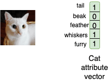
Semantic embedding using attribute vector — Figure 1 An example of semantic embedding using attribute vector

In the example shown above, the image is $x$ , the class label $y$ is “cat”, and the auxiliary information $h_y$ is stored as a binary vector consisting of 5 elements — tail, beak, feather, whiskers, furry. A cat has a tail, and is furry and therefore the binary encoding is 1 in the bins corresponding to tail and furry, and zero elsewhere.

Note that we will refer to this vector $h_y$ as semantic encoding for class $y$ in this post because it describes the class $y$ in words. The binary vector shown above is called an attribute vector and it is widely used for semantic encoding. However, there can be other kinds of semantic encodings as well.

Furthermore, mathematically we can say $y \in Y^S$ which simply means the class label can take a value of one of the seen classes ( $Y^S$ ) like “cat”, “dog” etc. Similarly, $x \in X^S$ where $X^S$ is the set of all seen images, and $h \in A^S$ where $A^S$ is the set of seen attributes.

Mathematically, this is written as

$S = \{ (x, y, h_y)|x \in X^S, y \in Y^S, h \in A^S \}$

Just so the notation does not scare you, let me write it in simple english. The above expression simply means, the collection of seen data consists of the image $x$ , the label $y$ , and the semantic encoding $h_y$ . The image is one of the images in the set $X^S$ , the label is one of the labels from the set $Y^S$ , and the encoding is from the set $A^S$ .

We also have the set of data for unseen classes denoted by $U$ . If you understood the above, you will also understand the following notation.

$U = \{ (x, y, h_y)|x \in X^U, y \in Y^U, h \in A^U \}$

Where, $X^U$ is the set of images with unseen images, $Y^U$ is the class of unseen labels (zebra in our example) and $A^U$ is the set of attributes for unseen classes.

Types of Zero-shot Learnings

The zero-shot learning problem can be divided into categories based on the data present during the training phase and testing phase-

Data present during training phase

Based on data available at the time of training a model, zero-shot learning can be divided into two categories.

Inductive Zero-shot

In this setting, we have access to labelled image data from seen classes i.e set $S$ during the training phase.

In addition to this, we also have access to semantic descriptions/attributes of both seen and unseen classes i.e the set $A^S \cup A^U$ during training.

The main goal in this setting is to transfer knowledge from semantic space to visual image space so that the model can recognize objects from unseen classes at test time.

Transductive Zero-shot

In the transductive setting, in addition to labelled image data from seen classes( i.e set $S$ ) we also have access to unlabelled images from unseen classes i.e set $X^U$ during the training phase.

Similar to inductive setting, semantic descriptions/attributes of both seen and unseen classes i.e the set $A^S \cup A^U$ are available during training.

This setting is useful in practical scenarios where we have access to a large pool of images but annotating/labelling each image is either not possible or labour intensive.

Compared to the inductive setting, the transductive setting is a bit easier as the model has some knowledge about the distribution of visual features of unseen classes.

Data present during testing phase

Based on the the data available at the time of testing or inference, we can divide zero-shot learning into two categories.

Conventional Zero-shot learning

In conventional zero-shot learning, the images to be recognized at test time belong only to unseen classes i.e test classes $\in Y^U$ .

This setting is practically less useful as in realistic scenarios, the assumption that the images at test time will come only from unseen classes is difficult to guarantee.

Generalized Zero-shot learning

In the generalized zero-short learning, the images at test time may belong to seen or unseen classes i.e test classes $\in Y^S \cup Y^U$ .

This setting is practically more useful/realistic and much more challenging than the conventional setting. The reason is that the model has been trained only on seen class images and therefore its predictions are biased towards seen classes. This leads to many unseen class images being wrongly classified into seen classes at test time which drastically reduces performance.

Challenges in Zero-shot learning

In order to get a deeper understanding of the zero-shot paradigm and formulate methods to solve the problem, it is important to understand the major challenges that zero-shot recognition.

Let us look at some challenges in zero-shot classification that play a major role in deciding the performance of a model.

Domain shift

In simple terms, domain shift refers to the problem where the training and testing data come from two different distributions.This plays an important role in zero-shot as almost always, the distribution of seen classes on which the model is trained is different from the distribution of unseen classes on which the model has to be tested.Since our deep network learns the function using only seen classes during training, it might not work for/generalize well to out of distribution unseen classes at test time.

Bias

In zero-shot learning, the model has access to only seen class image-label pairs during training and no unseen class images are available.This makes our model inherently biased towards predicting the seen classes as the correct class at test time.This problem becomes crucial especially in the case of generalized ZSL where the test image can belong to both seen or unseen classes.Since the model is biased towards seen classes, it often misclassifies unseen class images into one of the seen classes which reduces recognition performance drastically.

Cross-domain knowledge transfer

While training a zero-shot model, we have visual image features for seen classes and only semantic information for unseen classes. However, at test time we need to recognize visual features from unseen classes. Thus, how well our model is at knowledge transfer from semantic domain to visual domain plays a crucial role in zero-shot recognition.

For example, let us suppose that our model has seen a brown bear during training but not a polar bear. At test time, to recognize a polar bear our model needs to first transfer the ‘white fur’ attribute of a polar bear into visual space and merge it with the brown bear visual features to recognize a polar bear image correctly.

Semantic loss

While learning a classifier on seen classes during training, the model might attributes/features that do not help it to differentiate between seen classes. However, those ignored features could be helpful to differentiate between unseen classes at test time.

Let us understand this with an example. Suppose we have 2 classes — male and female at train time. Our model will learn to look for features like “facial appearance”, “body structure” etc to differentiate between male and female classes. The attribute “two legged” does not help it to differentiate between the classes and therefore it may not regard that attribute as important. But at test time if one of the novel unseen classes is dog, the information about the number of legs is very useful in distinguishing it from seen classes.

However, our model has learned to ignore the information about the number of legs since it was not useful at train time. In other words, we have experienced a “semantic loss” during the trining process.

Hubness

The problem of hubness arises when a high dimensional vector is projected into a low dimensional space. Such a projection reduces variance and results in mapped points being clustered as a hub.

Let us see how this affects zero-shot performance with an example. One of the most common approaches to address the zero-shot recognition problem is to learn a projection function from high dimensional visual space to low dimensional semantic space (discussed in detail later in the post). This leads to the formation of hubs of projected points in the semantic space. The points in these hubs tend to be near to semantic attribute vectors of large proportion of classes. Since at test time, we use a nearest neighbor search in semantic space, this leads to deterioration in performance.

Zero-shot Methodologies:

Let us now look into the details at two common approaches used to solve the zero-shot recognition problem

1. Embedding based methods

zero-shot-learning-embedding-based-methods – LearnOpenCV — Figure 2 Zero shot learning using Embedding based methods

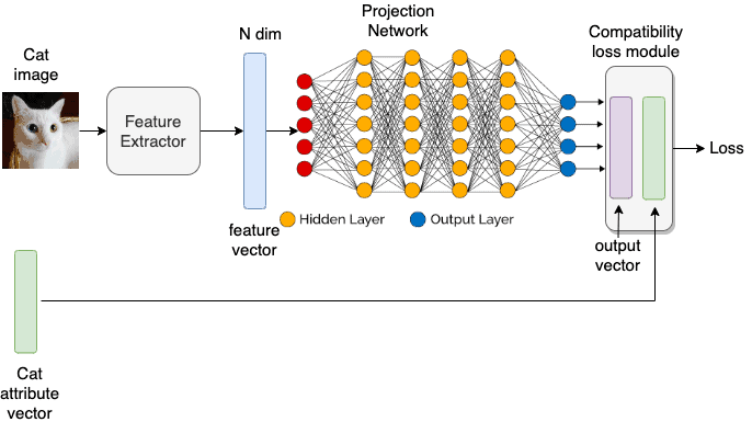
The main goal of embedding based methods is to map the image features and semantic attributes into a common embedding space using a projection function, which is learned using deep networks. The common embedding space can be the visual space, semantic space or a newly learned intermediate space.

Next, let us look at an example of one of these methods to understand it in depth.

Most embedding based methods use the semantic space as the common embedding space. During training, the aim is to learn a projection function from visual space (i.e image features) to semantic space (i.e word vectors/semantic embedding) using data from seen classes. Since, neural networks can be used as function approximators, the projection function is learned as a deep network.

During the test phase, the unseen class image features are passed as input to the trained network and we get the corresponding semantic embedding as the output. Thereafter, to perform classification, we do a nearest neighbour search in the semantic attribute space to find the closest match to the output of the network. Finally, the label corresponding to the closest semantic embedding is predicted as the output label of the input image feature.

The figure above shows the anatomy of a typical embedding based zero-shot method. The input image is first passed through a feature extractor network (typically a deep neural network) to get an N dimensional feature vector for the image. This feature vector acts as the input to our main projection network which in turn outputs a D dimensional output vector. The goal is to learn the weights/parameters of the projection network such that it maps the N dimensional input from visual space to a D dimensional output in the semantic space. To achieve this, we impose a loss which measures the compatibility between the D dim output and ground truth semantic attribute. The weights of the network are trained such that the D dim output is as close as possible to the ground truth attribute.

Generative model based methods

The main drawback with embedding based methods is that they suffer from the problem of bias and domain shift. This means that since the projection function is learned using only seen classes during training, it will be biased towards predicting seen class labels as the output. There is also no guarantee that the learned projection function will correctly map unseen class image features to the corresponding semantic space correctly at test time. This is due to the fact that the deep network has only learned to map seen class image features to semantic space during training and might not be able to do the same for novel unseen classes at test time correctly.

To overcome this drawback, it is necessary that out zero-shot classifier is trained on both seen and unseen class images at train time. This is where generative models based methods come in the picture. Generative methods aim to generate image features for unseen classes using the semantic attributes. Typically, this is done using a conditional generative adversarial network which generates image features conditioned on the semantic attribute of a particular class.

The figure below shows the block diagram of a typical generative model based zero-shot method. Similar to the embedding based method we use a feature extractor network to get an N dim feature vector. First, the attribute vector is input to the generative model as shown in the figure.The generator generates an N dim output vector conditioned on the attribute vector.The generative model is trained such that the synthesized feature vector looks indistinguishable from the original N dim feature vector.

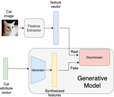
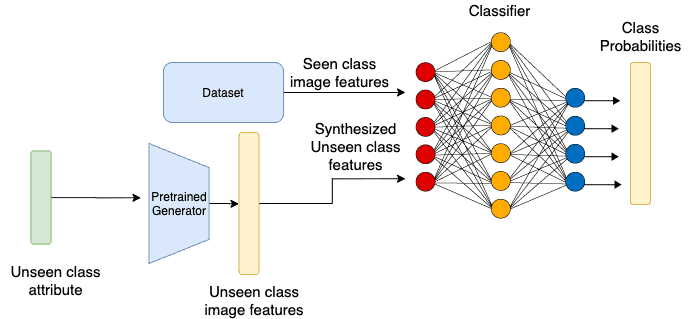
Figure 3 Obtaining image features from attribute vector using GAN

Once the generative model is trained, we freeze the weights of the generator and pass the unseen class attributes as input to it to generate unseen class image features. Now, since we have both seen class image features (from the dataset) and unseen class image features (generated by generator) we can train a simple classifier which takes as input the image features and outputs the corresponding label as shown in the figure.

Zero-shot learning using generative model based methods — Figure 4 Zero shot learning using generative model based methods

Evaluation Metric for Zero-shot learning algorithms

Most image recognition models use Top-1 accuracy as their evaluation metric. However, the evaluation protocol used for zero-shot recognition models is different from that used for vanilla image classification models.

To evaluate zero-shot performance we use the average per-class-top-1 accuracy instead. In simple words this means that we find the recognition accuracy for each class separately and then average it over all classes. This encourages high performance on both sparsely and densely populated classes. Mathematically, for a set of classes $Y$ with $N$ classes, the average per-class-top-1 accuracy $a_{Y}$ is given by

(1) $\begin{align*}a_{Y} = \frac{1}{N}\sum_{c=1}^{N} \frac{\textrm{\# of correct predictions in }c}{\textrm{\# of samples in } c}\end{align*}$

In case of generalized zero-shot setting, we aim for high accuracy on both seen classes Y^S as well as set of unseen classes Y^U.Thus the performance metric is defined as the harmonic mean of performance on seen classes and unseen classes.Mathematically,

(2) $\begin{align*}H = \frac{2 \times a_{Y^U} \times a_{Y^S}} {a_{Y^U} + a_{Y^S}}\end{align*}$

If you liked this article, please subscribe to our newsletter. You will also receive a free Computer Vision Resource guide. In our newsletter, we share Computer Vision, Machine Learning and AI tutorials written in Python and C++ using OpenCV, Dlib, Keras, Tensorflow, CoreML, and Caffe.

Subscribe Now