Variational Autoencoder in TensorFlow (Python Code)

Demo of Variational Autoencoder in TensorFlow

Deep Learning has already surpassed human-level performance on image recognition tasks. On the other hand, in unsupervised learning, Deep Neural networks like Generative Adversarial Networks ( GANs ) have been quite popular for generating realistic synthetic images and various other applications. Before GAN was invented, there were various fundamental and well-known Neural-Network based Architectures for Generative Modeling. And today, we will take you back in time and discuss one of the most popular pre-GAN eras Deep Generative Model known as Variational Autoencoder. In this tutorial, you will be introduced to Variational Autoencoder in TensorFlow.

In our previous post, we introduced you to Autoencoders and covered various aspects of it both theoretically and practically. We learned why autoencoders are not purely generative in nature; they are only good at generating images when you manually pick points in latent space and feed through the decoder. We validated our hypothesis by experimenting with Autoencoders on two datasets: Fashion-MNIST and Google’s Cartoon Set Data.

Do check out the post Introduction to Autoencoder in TensorFlow, if you haven’t already!

In this blog post we cover the following

Introduction to Variational Autoencoder, and how it overcomes the caveats in vanilla autoencoder?
Discuss the Loss Function of Variational Autoencoder.
Train a variational autoencoder using Tensorflow on Fashion MNIST
Train a variational autoencoder using Tensorflow on Google’s cartoon Dataset
- The Dataset
- The Network
Visualize the latent space of both trained variational autoencoders.
Reconstruction: Generate Synthetic Images sampled from the latent-space:
- Uniform Distribution
- Normal Distribution
Conclusion

With the experiments mentioned in points 4, 5, and 6, we will see that the variational autoencoder is better at learning the data distribution and can generate realistic images from a normal distribution compared to the vanilla autoencoder.

Introduction to Variational Autoencoder

ae-vae-revise – LearnOpenCV — An Autoencoder

From our previous post on Autoencoder, we discovered that given an input image $X$ , the encoder $G$ parameterized with $\theta$ learned to map the input into a fixed latent-vector $Z$ . From the latent-vector $Z$ the decoder $F$ parameterized with $\phi$ learned to reconstruct the image $\hat{X}$ similar to input-image $X$ . To achieve this we minimized a reconstruction loss i.e. mean-squared error given as $\frac{1}{N}\sum_{i=1}^{N}{(X_i -\hat{X_i})^2}$ where $N$ was the number of images in a batch.

The latent-space $Z$ in Autoencoder was also known as a bottleneck since the dimension of $Z$ was smaller than the input $X$ . In other words, Encoder-Decoder models were jointly trained to minimize reconstruction loss. We learned an encoding $Z$ given an input $X$ such that the reconstructed output $\hat{X}$ from given $Z$ looked similar to the input.

However, Autoencoder was not good at generating new images since its primary issue was in the latent space structure. The latent space was not continuous and did not allow easy interpolation. Encoded vectors were grouped in clusters corresponding to different data classes, and there were huge gaps between the clusters. While generating a new sample, the decoder often produced a gibberish output if the chosen point in the latent space did not contain any data.

Without further ado, let’s get straight into Variational Autoencoder.

Architecture of Variational Autoencoder in TensorFlow — Variational Autoencoder

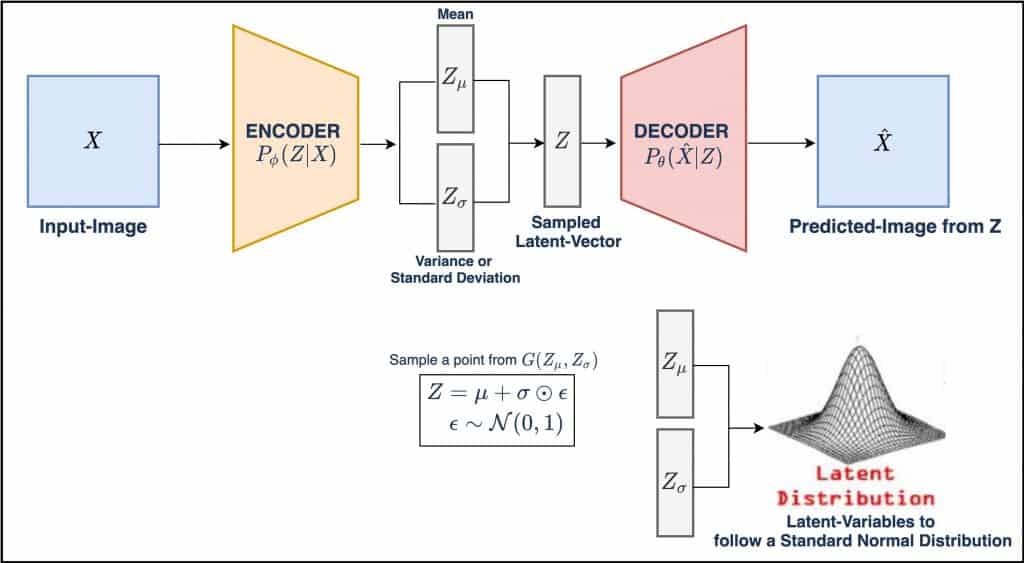
Variational Autoencoder ( VAE ) came into existence in 2013, when Diederik et al. published a paper Auto-Encoding Variational Bayes. This paper was an extension of the original idea of Auto-Encoder primarily to learn the useful distribution of the data. Variational Autoencoder was inspired by the methods of the variational bayesian and graphical model. VAE is rooted in Bayesian inference, i.e., it wants to model the underlying probability distribution of data to sample new data from that distribution.

VAE has one fundamentally unique property that separates them from vanilla autoencoder, and it is this property that makes them so useful for generative modeling: their latent spaces are, by design, continuous, allowing easy random sampling and interpolation.

Throughout the tutorial we will refer to Variational Autoencoder by VAE.

Variational Autoencoder (VAE) is a generative model that enforces a prior on the latent vector. The latent vector has a certain prior i.e. the latent vector $Z$ should have a Multi-Variate Gaussian profile ( prior on the distribution of representations ). Instead of mapping the image on a point in space, the encoder of VAE maps the image onto a normal distribution.

In the above figure, the input image is fed to the encoder, which outputs two latent variables $Z_{\mu}$ and $Z_{\sigma}$ which are the parameters of the distribution that you learn during the training. Instead of directly outputting a latent-space $Z$ that is not enforced to follow any distribution, in VAE, we have two latent variable $Z_{\mu}$ and $Z_{\sigma}$ from which you sample a latent-vector $Z$ . The sampled latent-vector $Z$ can also be called a sampling-layer which samples from a Multi-Variate Gaussian $G(Z_{\mu}, Z_{\sigma})$ where $Z_{\mu}$ and $Z_{\sigma}$ are the mean and variances respectively. We pass the sampled vector $Z$ to the decoder and obtain the predicted image $\hat{X}$ .

As discussed, we want our latent vector $Z$ to follow a standard normal distribution and to achieve that the variables $Z_{\mu}$ and $Z_{\sigma}$ are trained such that $Z_{\mu}$ is close to zero and $Z_{\sigma}$ is near to 1.

encodings-vae – LearnOpenCV — <a href=httpstowardsdatasciencecomintuitively understanding variational autoencoders 1bfe67eb5daf target= blank rel=noreferrer noopener>Image Source<a>

Instead of a single point in the latent space as in vanilla autoencoder, the VAE covers a certain “area” centered around the mean value with a size corresponding to the standard deviation. This gives the decoder a lot more to work with — a sample from anywhere in the area will be very similar to the original input.

How do we achieve latent variables $Z_{\mu}$ and $Z_{\sigma}$ ?

Assume the encoder has convolutional layers and the last convolutional layer output is flattened into a vector; let’s call it flat_out. The flat_out is fed to two separate dense layers ( for example, having N neurons each) $Z_{\mu}$ and $Z_{\sigma}$ . The size of both $Z_{\mu}$ and $Z_{\sigma}$ would then be [N, 1]. Don’t worry if it is a bit confusing since it would be a lot clear in the coding section.

In VAE, the latent variable $Z_{\sigma}$ is assumed to not correlate with any of the latent space dimensions and the diagonal matrix has a closed-form and is easy to implement. So we consider only the diagonal elements of the covariance matrix i.e. the variance or standard deviation elements.

Hence, a conventional VAE encoder assuming Gaussian distribution for a single data point produces latent parameters $Z_{\mu}$ and $Z_{\sigma}$ . There are $N$ elements in each of $Z_{\mu}$ and $Z_{\sigma}$ so the total number of latent parameters is $2N$ .

Why Normal/Gaussian Distribution?

We assume that our dataset would inherently follow a distribution similar to the normal distribution. Enforcing the latent variables to follow a normal distribution in VAE is very common and works the best. However, some work in VAEs uses Gaussian mixtures, Bernoulli, and von Mises-Fisher distribution. The normal distribution has many properties that favor the training of VAE, such as analytical evaluation of the KL divergence in the variational loss, use of the reparametrization trick for efficient gradient computation. You can generate new images by sampling with latent variables $Z_{\mu}$ and $Z_{\sigma}$ , and you can also generate new images by simply sampling from a standard normal distribution after VAE is trained.

Comparing VAE structure with Autoencoder from the above figure we say that:

The approximation function $P_{\phi}(Z|X)$ is the probabilistic encoder, playing a similar role as the vanilla autoencoder’s encoder.
The conditional probability $P_{\theta}(\hat{X}|Z)$ defines a generative model also known as a probabilistic decoder, it is similar to the plain autoencoder’s decoder.

VAE Objective

In VAE, we optimize two loss functions: reconstruction loss and KL-divergence loss. We will learn about them in detail in the next section. For now, remember that the reconstruction loss ensures that the images generated by the decoder are similar to the input or the ones in the dataset. While the KL-divergence measures the divergence between a pair of probability distributions, in this case, the pair of distributions being the latent vector $Z$ ( sampled from $Z_{\mu}$ and $Z_{\sigma}$ ) and unit normal distribution $\mathcal{N}(0, 1)$ . KL-divergence ensures that the latent-variables are close to the standard normal distribution.

Generation of Samples in VAE after Training

Well, once your model is trained, during the test time, you basically sample a point from the standard normal distribution, and pass it through the decoder, which then generates an image similar to the ones in the dataset. The decoder part of VAE can be termed as “generative” since it learns to generate diverse, realistic images sampled from the Gaussian distribution.

Objective Function of VAE

Till now, we learned that in VAE, we constrain our encoder network to generate a latent vector $Z$ ( sampled from $Z_{\mu}$ and $Z_{\sigma}$ ) that roughly follows:

Unit Gaussian Distribution $\mathcal{N}(0, 1)$ , and
Minimize the reconstruction error $\frac{1}{N}\sum_{i=1}^{N}{(X_i -\hat{X_i})^2}$ .

VAE’s loss function comprises a Reconstruction error, and a KL-divergence error used to model the networks’ objectives. The final loss is a weighted sum of both losses.

VAE’s total loss can be given as:

(1) $\begin{equation*}$L(\phi, \theta, x) = (reconstruction-loss) + (regularization-term)$ \end{equation*}$

(2) $\begin{equation*}$L(\phi, \theta, x) = \frac{1}{N}\sum_{i=1}^{N}{(X_i -\hat{X_i})^2} + KL[G(Z_{\mu}, Z_{\sigma}), \mathcal{N}(0, 1)]$ \end{equation*}$

Reconstruction Error

The reconstruction loss in VAE is similar to the Loss we used in Autoencoder i.e. Mean-Squared-Error often called MSE.

Reconstruction loss ensures that the input image is reconstructed at the output, and by doing so, the loss inherently makes the encoding and the decoding of VAE efficient and meaningful. The goal of VAE is to not only learn the distribution but also produce realistic-looking images similar to the training data. Hence, we need a reconstruction error function.

The reconstruction loss is given as:

(3) $\begin{equation*}L_{MSE}(\theta ,\phi ) = \frac{1}{N}\sum_{i=1}^{N}{\Big(x_i -f_\theta (g_\phi (x_i))\Big)^2} \end{equation*}$

where $\theta$ and $\phi$ are the parameters of the encoder and decoder, respectively. $N$ is the number of images in your dataset or the mini-batch across which the loss is computed. MSE computes the pixel-wise difference between the original and the reconstructed output, raises the difference to the power of two, and takes an average over the full-batch or mini-batch of the data.

MSE using numpy can be written as:

MSE = numpy.mean((X - X_hat)**2)

Here $X$ is the input image fed to the encoder, and $\hat{X}$ is the predicted image from $Z$ ( decoder ) of VAE.

KL Divergence

Recall in VAE we would like the image encodings to be as close as possible to each other while still be unique, allowing for the generation of samples that looks similar to the real ones with smooth interpolation in the latent space. To achieve all of this we introduce a new loss function in VAE known as Kullback-Leibler Divergence.

Kullback–Leibler Divergence ( KL Divergence ) is a measure of how one probability distribution differs from a second, reference probability distribution.

In VAE, our primary objective is to learn the underlying data distribution so that we can generate new data samples from that distribution. VAE is a parametric model in which we assume the distribution and distribution parameters like $\mu$ and $\sigma$ , and we try to estimate that distribution. To estimate a distribution, we need to assume that data comes from a specific distribution like Gaussian, Bernoulli, etc. Hence, in VAE, the assumption is that the data distribution is Gaussian.

We train our VAE to minimize the KL divergence between the encoder’s distribution $P_{\phi}(Z|X)$ and $P(Z)$ . In VAE, $P(Z)$ follows a standard or unit Normal distribution ( $\mu = 0$ and $\sigma = 1$ ) or $P(Z) = \mathcal{N}(0, 1)$ . If the encoder outputs encoding $Z$ far from a standard normal distribution, KL-divergence loss will penalize it more. The KL-divergence acts as a regularize, which keeps the encodings $Z$ sufficiently diverse. If we omitted the regularizer, the encoder could learn to cheat and give each datapoint an encoding in a different Euclidean space region. In other words, KL divergence optimizes the probability distribution parameters $\mu$ and $\sigma$ to closely resemble the unit gaussian distribution $\mathcal{N}(0, 1)$ .

In a VAE, we want to measure how different our normal distribution with parameters $\mu$ and $\sigma$ are from a unit normal distribution. While calculating the KL-divergence we choose to map the parameter $\sigma^2$ ( variance ) to the logarithm of the variance. By taking the logarithm of the variance, we force the network to have the output range of the natural numbers rather than just positive values (variances would only have positive values). This allows for smoother representations for the latent space.

In this special case, the KL divergence has the closed form:

(4) $\begin{equation*}L_{KL}[G(Z_{\mu}, Z_{\sigma}) \| \mathcal{N}(0, 1)] = - 0.5 * \sum_{i=1}^{N}{1 + log(Z_{\sigma_{i}}^2}) - Z_{\mu_{i}}^2 - e^{log(Z_{\sigma_{i}}^2)}} \end{equation*}$

The eq. 3 can be rewritten as:

(5) $\begin{equation*}L_{KL}[G(Z_{\mu}, Z_{\sigma}) \| \mathcal{N}(0, 1)]= - 0.5 * \sum_{i=1}^{N}{1 + log(Z_{\sigma_{i}}^2}) - Z_{\mu_{i}}^2 - Z_{\sigma_{i}}^2} \end{equation*}$

In the above equation $Z_{\mu}$ and $Z_{\sigma}^2$ are the mean and variance vectors of the encoder’s latent-space. And the sum is taken over all the dimensions in the latent space.

KL-divergence in numpy can be written as:

kl_loss =  -0.5 * numpy.sum(1 + numpy.log(Z_sigma ** 2) - numpy.square(Z_mean) - numpy.exp(np.log(Z_sigma ** 2), axis = 1)

kl_loss =  -0.5 * numpy.sum(1 + numpy.log(Z_sigma ** 2) - numpy.square(Z_mean) - Z_sigma ** 2, axis = 1)

Reparameterization Trick

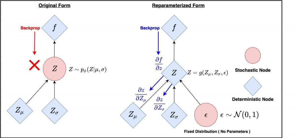
The above figure shows two computation graphs: the original form ( left ) and the reparameterized form ( right ). $Z_\mu$ and $Z_\sigma$ represent the parameters the network tries to learn. The deterministic nodes, i.e., input and weights, are shown in blue, while the stochastic nodes are represented in red.

In this diagram, during the training, the image $X$ is mapped to two latent-variables $Z_{\mu}$ and $Z_{\sigma}$ and we sample a vector $Z$ from the two latent variables which are fed to the decoder to output an image $\hat{X}$ . However, this stochastic sampling operation makes $Z$ a random node which creates a bottleneck because gradients cannot backpropagate through the sampling layer because of its stochastic nature. As a result of which the parameters $Z_\mu$ and $Z_\sigma$ cannot learn. Backpropagation requires the nodes to be deterministic to iteratively pass gradients through and apply the chain rule.

To address this issue a reparameterization trick was introduced in VAE which converted the random node $Z$ to a deterministic node. This allowed the $Z_\mu$ and $Z_\sigma$ vectors to remain as the learnable parameters of the network while still maintaining the stochasticity of the entire system via $\varepsilon$ .

Instead of sampling vector $Z$ from a normal distribution parameterized by $\mu$ and $\sigma$ ( $Z \sim \mathcal{N}(Z_\mu, Z_\sigma^2)$ ) which did not allow us to compute the gradients we approximate the sampled latent vector $Z$ as a sum of

a fixed mean vector $\mu$ , and
a fixed standard deviation vector $\sigma$ , scaled by random constants drawn from the prior distributions i.e. unit gaussian distribution.

The new sampling operation can be written as:

(6) $\begin{equation*} $Z = Z_\mu + Z_\sigma^2 \odot \varepsilon \end{equation*}$

Here, $\varepsilon \sim \mathcal{N}(0, 1)$ and $\odot$ is element-wise multiplication.

Now even after reparameterization we still have the stochasticity preserved or the stochastic node but since now we added the $\varepsilon$ drawn from a unit gaussian, hence, the stochastic sampling does not happen in the latent-space layer $Z$ .

Let’s now move onto implementing a variational autoencoder for generating Fashion-MNIST and Cartoon images in TensorFlow.

Coding a Variational Autoencoder in TensorFlow

Dataset

We will use the famous Fashion-MNIST dataset for this purpose.

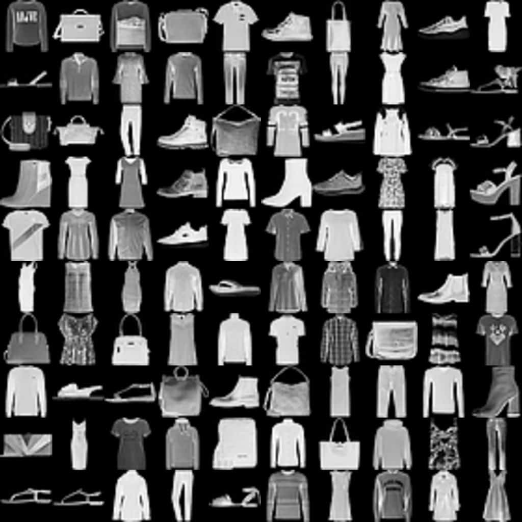
The Fashion-MNIST dataset consists of:

Database of 60,000 fashion images shown on the right.
Each image of size 28×28 ( grayscale ) is associated with a label from 10 categories like t-shirt, trouser, sneaker, etc.

Note: All the implementations were carried out on an 11GB Pascal 1080Ti GPU.

Download Code To easily follow along this tutorial, please download code by clicking on the button below. It's FREE!

Click here to download the source code to this post

Importing Modules

# import the necessary packages
import imageio
import glob
import os
import time
import cv2
import tensorflow as tf
from tensorflow.keras import layers
from IPython import display
import matplotlib.pyplot as plt
import numpy as np
%matplotlib inline
from tensorflow import keras

We begin by importing necessary packages like imageio, glob, tensorflow, tensorflow layers, time, and matplotlib for plotting on Lines 2-10.

Loading and Preprocessing Dataset

(x_train, y_train), (x_test, y_test) = tf.keras.datasets.fashion_mnist.load_data()
x_train = x_train.reshape(x_train.shape[0], 28, 28, 1).astype('float32')
x_test = x_test.astype('float32')
x_train = x_train / 255.
x_test = x_test / 255.
# Batch and shuffle the data
train_dataset = tf.data.Dataset.from_tensor_slices(x_train).\
shuffle(60000).batch(128)

Loading the dataset is fairly simple; you can use the tf_keras datasets module, which loads the data off-the-shelf. Since we do not require the labels to solve this problem, we will use the training images x_train. In Line 15, you reshape the images and cast them to float32 since the data is inherently in uint8 format.

Then, in Line 17-18, you normalize the data from [0, 255] to [0, 1]. Finally, we build the TensorFlow input pipeline. In short, tf.data.Dataset.from_tensor_slices is fed the training data, shuffled, sliced into tensors, allowing you to access tensors of specified batch size during training. The buffer size ( 60000 ) parameter in shuffle affects the randomness of the shuffle.

Architectural Diagram of Autoencoder

Define the Encoder Network

def encoder(input_encoder):
  
    inputs = keras.Input(shape=input_encoder, name='input_layer')

    # Block-1
    x = layers.Conv2D(32, kernel_size=3, strides= 1, padding='same', name='conv_1')(inputs)
    x = layers.BatchNormalization(name='bn_1')(x)
    x = layers.LeakyReLU(name='lrelu_1')(x)
    
    # Block-2
    x = layers.Conv2D(64, kernel_size=3, strides= 2, padding='same', name='conv_2')(x)
    x = layers.BatchNormalization(name='bn_2')(x)
    x = layers.LeakyReLU(name='lrelu_2')(x)
    
    # Block-3
    x = layers.Conv2D(64, 3, 2, padding='same', name='conv_3')(x)
    x = layers.BatchNormalization(name='bn_3')(x)
    x = layers.LeakyReLU(name='lrelu_3')(x)
  
    # Block-4
    x = layers.Conv2D(64, 3, 1, padding='same', name='conv_4')(x)
    x = layers.BatchNormalization(name='bn_4')(x)
    x = layers.LeakyReLU(name='lrelu_4')(x)
   
    # Final Block
    flatten = layers.Flatten()(x)
    mean = layers.Dense(2, name='mean')(flatten)
    log_var = layers.Dense(2, name='log_var')(flatten)
    model = tf.keras.Model(inputs, (mean, log_var), name="Encoder")
    return model

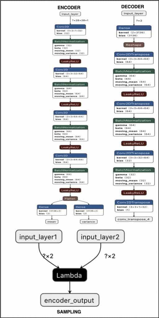
Here we define the encoder network which takes an input of size [None, 28, 28, 1]. There are a total of four Conv blocks each consisting of a Conv2D, BatchNorm and LeakyReLU activation function. In each block, the image is downsampled by a factor of two. The slope of LeakyReLU is by default 0.2.

In the final block or the Flatten layer we convert the [None, 7, 7, 64] to a vector of size 3136.

Pay attention to Lines 48-49 since this is where we define mean and log_variance vectors. These two vectors are also known as latent-variables. The output of the model will be passed to the sampling network. The Network ( encoder ) learns to map the data ( Fashion-MNIST ) to two latent variables ( mean & variance vectors ) that are expected to follow a normal distribution.

The Sampling Network

def sampling(input_1,input_2):
    mean = keras.Input(shape=input_1, name='input_layer1')
    log_var = keras.Input(shape=input_2, name='input_layer2')
    out = layers.Lambda(sampling_reparameterization_model, name='encoder_output')([mean, log_var])
    enc_2 = tf.keras.Model([mean,log_var], out,  name="Encoder_2")
    return enc_2

Now we define a second network that takes mean and variance tensors as input. It has a Lambda layer which calls a function sampling_reparameterization_model and passes mean and variance tensors to it. A Lambda layer comes in handy when you want to pass a tensor to a custom function that isn’t already included in tensorflow.

def sampling_reparameterization(distribution_params):
    mean, log_var = distribution_params
    epsilon = K.random_normal(shape=K.shape(mean), mean=0., stddev=1.)
    z = mean + K.exp(log_var / 2) * epsilon
    return z

The above sampling_reparameterization is called by the sampling function which is fed the output of the encoder i.e. mean and variance. During the training phase, the above function samples a z vector, which is then fed as an input to the decoder.

As we learned earlier that sampling from the latent distribution defined by the parameters ( mean & log_variance ) outputted by the encoder creates a bottleneck as backpropagation cannot flow from a non-deterministic node.

To address this, we use a reparameterization trick which allows the loss to backpropagate through the mean and variance nodes since they are deterministic while separating the sampling node by adding a non-deterministic parameter eps. This makes z deterministic and backpropagation works like a charm. The eps can be thought of as a random noise used to maintain the required stochasticity of z. Here the eps is sampled from a standard normal distribution ( mean=0., stddev=1. ).

Note in the above function, we output log-variance instead of the variance to maintain numerical stability.

Define the Decoder Network

def decoder(input_decoder):
    
    inputs = keras.Input(shape=input_decoder, name='input_layer')
    x = layers.Dense(3136, name='dense_1')(inputs)
    x = layers.Reshape((7, 7, 64), name='Reshape_Layer')(x)
   
    # Block-1
    x = layers.Conv2DTranspose(64, 3, strides= 1, padding='same',name='conv_transpose_1')(x)
    x = layers.BatchNormalization(name='bn_1')(x)
    x = layers.LeakyReLU(name='lrelu_1')(x)
  
    # Block-2
    x = layers.Conv2DTranspose(64, 3, strides= 2, padding='same', name='conv_transpose_2')(x)
    x = layers.BatchNormalization(name='bn_2')(x)
    x = layers.LeakyReLU(name='lrelu_2')(x)
    
    # Block-3
    x = layers.Conv2DTranspose(32, 3, 2, padding='same', name='conv_transpose_3')(x)
    x = layers.BatchNormalization(name='bn_3')(x)
    x = layers.LeakyReLU(name='lrelu_3')(x)
    
    # Block-4
    outputs = layers.Conv2DTranspose(1, 3, 1,padding='same', activation='sigmoid', name='conv_transpose_4')(x)
    model = tf.keras.Model(inputs, outputs, name="Decoder")
    return model

The decoder network of the variational autoencoder is exactly similar to a vanilla autoencoder. It takes an input of size [None, 2]. The initial block has a Dense layer having 3136 neurons, recall in the encoder function this was the size of the vector after flattening the output from the last conv block. There are a total of four Conv blocks. The Conv block [1, 3] consists of a Conv2DTranspose, BatchNorm and LeakyReLU activation function. The Conv block 4 has a Conv2DTranspose with sigmoid activation function, which squashes the output in the range [0, 1] since the images are normalized in that range. In each block, the image is upsampled by a factor of two.

The output from the decoder network is a tensor of size [None, 28, 28, 1].

Optimizer and Loss Function

optimizer = tf.keras.optimizers.Adam(lr = 0.0005)

def mse_loss(y_true, y_pred):
    r_loss = K.mean(K.square(y_true - y_pred), axis = [1,2,3])
    return 1000 * r_loss

def kl_loss(mean, log_var):
    kl_loss =  -0.5 * K.sum(1 + log_var - K.square(mean) - K.exp(log_var), axis = 1)
    return kl_loss

def vae_loss(y_true, y_pred, mean, var):
    r_loss = mse_loss(y_true, y_pred)
    kl_loss = kl_loss(mean, log_var)
    return  r_loss + kl_loss

Training the Variational Autoencoder

# Notice the use of `tf.function`
# This annotation causes the function to be "compiled".
@tf.function
def train_step(images):

    with tf.GradientTape() as encoder, tf.GradientTape() as decoder:
      
        mean, log_var = enc(images, training=True)
        latent = sampling([mean, log_var])
        generated_images = dec(latent, training=True)
        loss = vae_loss(images, generated_images, mean, log_var)

        
    gradients_of_enc = encoder.gradient(loss, enc.trainable_variables)
    gradients_of_dec = decoder.gradient(loss, dec.trainable_variables)
    
    
    optimizer.apply_gradients(zip(gradients_of_enc, enc.trainable_variables))
    optimizer.apply_gradients(zip(gradients_of_dec, dec.trainable_variables))
    return loss

In the above training loop, we train the encoder and decoder separately. There is a third model, i.e., the sampling model whose job is to sample a z given the mean and log_variance vectors, there is no learning that happens in the sampling model. We first pass the image to the encoder, then the latent variables mean and variance are fed to the sampling model and the output latent is finally fed to the decoder. The loss is computed over the images generated by the decoder.

Next, in Line 119-120, we compute the gradients and update the encoder & decoder parameters using the Adam optimizer. Finally, we return the loss.

def train(dataset, epochs):
  for epoch in range(epochs):
    start = time.time()
    for image_batch in dataset:
      train_step(image_batch)

    print ('Time for epoch {} is {} sec'.format(epoch + 1, time.time()-start))


train(train_dataset, epoch)

Finally, we train our Autoencoder model. The above train function takes the train_dataset and Epochs as the parameters and calls the train_step function at every new batch in total $469$ ( Total Training Images / Batch Size).

Reconstructing Test Images

Let’s now test how well the model has learned to reconstruct the fashion images. We will use the test images, which are normalized in the range [0, 1]. We use Matplotlib to plot the images.

With every reconstructed output, we will also plot their respective ground truth or label to judge the reconstructed images’ quality.

figsize = 15

m, v = enc.predict(x_test[:25])
latent = sampling([m,v])
reconst = dec.predict(latent)

fig = plt.figure(figsize=(figsize, 10))

for i in range(25):
    ax = fig.add_subplot(5, 5, i+1)
    ax.axis('off')
    ax.text(0.5, -0.15, str(label_dict[y_test[i]]), fontsize=10, ha='center', transform=ax.transAxes)
    
    ax.imshow(reconst[i, :,:,0]*255, cmap = 'gray')

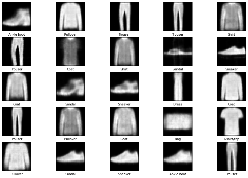
From the above output, we can observe that the model did a decent job of reconstructing the test images ( validating from the labels ) even though the objective of Variational Autoencoder was to minimize not just the reconstruction error ( MSE ) but also the distribution error ( KL-divergence ).

We will do a couple of more tests with our Fashion-MNIST Variational Autoencoder in the later part of the tutorial. Feel free to jump directly to that.

Variational Autoencoder with Cartoon Set Data

This section will only show the data loading, data preprocessing, encoder and decoder architecture since all other implementation parts are similar to the Fashion-MNIST implementation.

Dataset

Cartoon Set is a collection of random 2D cartoon avatar RGB images. The cartoons vary in 10 artwork categories, 4 color categories, and 4 proportion categories, with ~10¹³ possible combinations. The dataset consists of fixed-size images i.e., 512 x 512 x 3. The dataset comprises of two sets: 10k and 100k randomly chosen cartoons and labeled attributes. We would be using the 100k image set for training the Variational Autoencoder.

Loading and Preprocessing the Data

train_ds = tf.keras.preprocessing.image_dataset_from_directory(
  'cartoonset100k',
  image_size=(256, 256),
  batch_size=batch_size,
  label_mode=None)

normalization_layer = layers.experimental.preprocessing.Rescaling(scale= 1./255)

normalized_ds = train_ds.map(lambda x: normalization_layer(x))

Loading the dataset is fairly simple; you can use the tf_keras preprocessing dataset module, which has a function image_dataset_from_directory that loads the data from the specified directory, which in our case is cartoonset100k. We pass the desired image_size [256, 256, 3], batch_size = 128, and label_mode = None since this is an unsupervised problem.

Finally, in Line 9, we use the Lambda function to normalize all the input images from [0, 255] to [0, 1] and get normalized_ds which we will use for training our model. In the Lambda function, we pass the preprocessing layer defined at Line 7.

Variational Autoencoder Architecture

Define the Encoder Network

def encoder(input_encoder):
    
    
    inputs = keras.Input(shape=input_encoder, name='input_layer')
    
    # Block-1
    x = layers.Conv2D(32, kernel_size=3, strides= 2, padding='same', name='conv_1')(inputs)
    x = layers.BatchNormalization(name='bn_1')(x)
    x = layers.LeakyReLU(name='lrelu_1')(x)
  
    # Block-2
    x = layers.Conv2D(64, kernel_size=3, strides= 2, padding='same', name='conv_2')(x)
    x = layers.BatchNormalization(name='bn_2')(x)
    x = layers.LeakyReLU(name='lrelu_2')(x)
   
    # Block-3
    x = layers.Conv2D(64, 3, 2, padding='same', name='conv_3')(x)
    x = layers.BatchNormalization(name='bn_3')(x)
    x = layers.LeakyReLU(name='lrelu_3')(x)
   
    # Block-4
    x = layers.Conv2D(64, 3, 2, padding='same', name='conv_4')(x)
    x = layers.BatchNormalization(name='bn_4')(x)
    x = layers.LeakyReLU(name='lrelu_4')(x)
  
    # Block-5
    x = layers.Conv2D(64, 3, 2, padding='same', name='conv_5')(x)
    x = layers.BatchNormalization(name='bn_5')(x)
    x = layers.LeakyReLU(name='lrelu_5')(x)
 

    # Final Block
    flatten = layers.Flatten()(x)
    mean = layers.Dense(200, name='mean')(flatten)
    log_var = layers.Dense(200, name='log_var')(flatten)
    model = tf.keras.Model(inputs, (mean, log_var), name="Encoder")
    return model

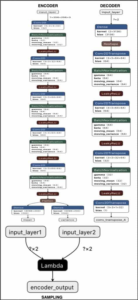
The encoder network takes an input of size [None, 256, 256, 3]. It consists of five Conv blocks each block has a Conv2D, BatchNorm and LeakyReLU activation function. In each block, the image is downsampled by a factor of two.

In Lines 43-44 we define the mean and variance vectors. These two vectors are also known as latent-variables. The output of the model will be fed to the sampling network. The Network ( encoder ) learns to map the data ( Fashion-MNIST ) to two latent variables ( mean & variance vectors ) that are expected to follow a normal distribution.

We can also say that an image of size 256 x 256 x 3 is encoded or represented by a mean & log_variance vector of size 200.

The Decoder Network

def decoder(input_decoder):
    
    inputs = keras.Input(shape=input_decoder, name='input_layer')
    x = layers.Dense(4096, name='dense_1')(inputs)
    x = layers.Reshape((8,8,64), name='Reshape')(x)
    
    # Block-1
    x = layers.Conv2DTranspose(64, 3, strides= 2, padding='same',name='conv_transpose_1')(x)
    x = layers.BatchNormalization(name='bn_1')(x)
    x = layers.LeakyReLU(name='lrelu_1')(x)
   
    # Block-2
    x = layers.Conv2DTranspose(64, 3, strides= 2, padding='same', name='conv_transpose_2')(x)
    x = layers.BatchNormalization(name='bn_2')(x)
    x = layers.LeakyReLU(name='lrelu_2')(x)
 
    # Block-3
    x = layers.Conv2DTranspose(64, 3, 2, padding='same', name='conv_transpose_3')(x)
    x = layers.BatchNormalization(name='bn_3')(x)
    x = layers.LeakyReLU(name='lrelu_3')(x)
   
    # Block-4
    x = layers.Conv2DTranspose(32, 3, 2, padding='same', name='conv_transpose_4')(x)
    x = layers.BatchNormalization(name='bn_4')(x)
    x = layers.LeakyReLU(name='lrelu_4')(x)

  
    # Block-5
    outputs = layers.Conv2DTranspose(3, 3, 2,padding='same', activation='sigmoid', name='conv_transpose_5')(x)
    model = tf.keras.Model(inputs, outputs, name="Decoder")
    return model

We learned that the decoder network of the variational autoencoder is similar to a vanilla autoencoder. It takes an input of size [None, 200]. The initial block has a Dense layer having 4096 neurons. There are a total of five Conv blocks. The Conv block [1, 4] consists of a Conv2DTranspose, BatchNorm and LeakyReLU activation function. The Conv block-5 has a Conv2DTranspose with sigmoid activation function, which squashes the output in the range [0, 1] since the images are normalized in that range. In each block, the image is upsampled by a factor of two.

The output from the decoder network is a tensor of size [None, 256, 256, 3].

Reconstructing the Cartoon Images

Let’s test our variational autoencoder model by reconstructing the cartoon images.

figsize = 15


fig = plt.figure(figsize=(figsize, 10))

for i in range(25):
    ax = fig.add_subplot(5, 5, i+1)
    ax.axis('off')
    pred = reconstruction[i, :, :, :] * 255
    pred = np.array(pred)  
    pred = pred.astype(np.uint8)
    
    ax.imshow(pred)

vae-cartoon-reconstruction – LearnOpenCV

Based on the above outputs, we can say that VAE did an excellent job reconstructing the cartoon images.

Visualizing the Latent Space

In this section, we will visualize VAE’s latent space trained on both Fashion-MNIST and Cartoon Set Data. We will compare the latent-space of vanilla autoencoder with VAE trained on cartoon set data. By visualizing both the latent-spaces, we will understand how VAE’s are different from Vanilla Autoencoder, primarily w.r.t the generation of images.

Latent Space Projection of Variational Autoencoder Trained on Fashion-MNIST

n_to_show = 5000
figsize = 12

example_idx = np.random.choice(range(len(x_test)), n_to_show)
example_images = x_test[example_idx]

m, v = enc.predict(example_images)
embeddings = sampling([m,v])

plt.figure(figsize=(figsize, figsize))
plt.scatter(embeddings[:, 0] , embeddings[:, 1], alpha=0.5, s=2)
plt.xlabel("Dimension-1", size=20)
plt.ylabel("Dimension-2", size=20)
plt.xticks(size=20)
plt.yticks(size=20)
plt.title("Projection of 2D Latent-Space (Fashion-MNIST)", size=20)
plt.show()

To plot the latent-space we randomly chose 5K images from the 10K test set of Fashion-MNIST and fed it to the encoder that outputs the mean and variance vectors. The two vectors were then fed to the sampling model outputting an embedding vector of shape [5000, 2]. We plot these 5K embeddings on x-axis and y-axis as shown in the above scatter plot.

Comparing this plot with the vanilla autoencoder plot from our last blog, we can see some pronounced differences. Firstly, the data points are bounded within a certain range; secondly, the range of both dimensions is minimal. Dimension-1 has values in the range [-3, 3], and Dimension-2 has values in the range [-4, 4]. The data points are symmetric around [0, 0], and the points are equally distributed in both positive and negative regions of the x-axis and y-axis.

The latent-space looks continuous; there are no gaps between the data points’ encodings. If we sample a point from a normal distribution, the decoder should generate an image similar to the point close by in the latent-space. However, in Autoencoder, because of the gaps and large boundaries, if you happened to pick a point from the gap where no data points were mapped and passed it to the decoder, it might have generated arbitrary output ( or noise ) that doesn’t resemble any of the classes.

The KL-divergence loss played a major role in ensuring that the mean and values follow a standard normal distribution. Since VAE was trained with such a constraint, you can therefore sample from the standard normal distribution and feed to the decoder to generate new images.

Latent Space Projection with t-SNE of VAE Trained on Cartoon Set

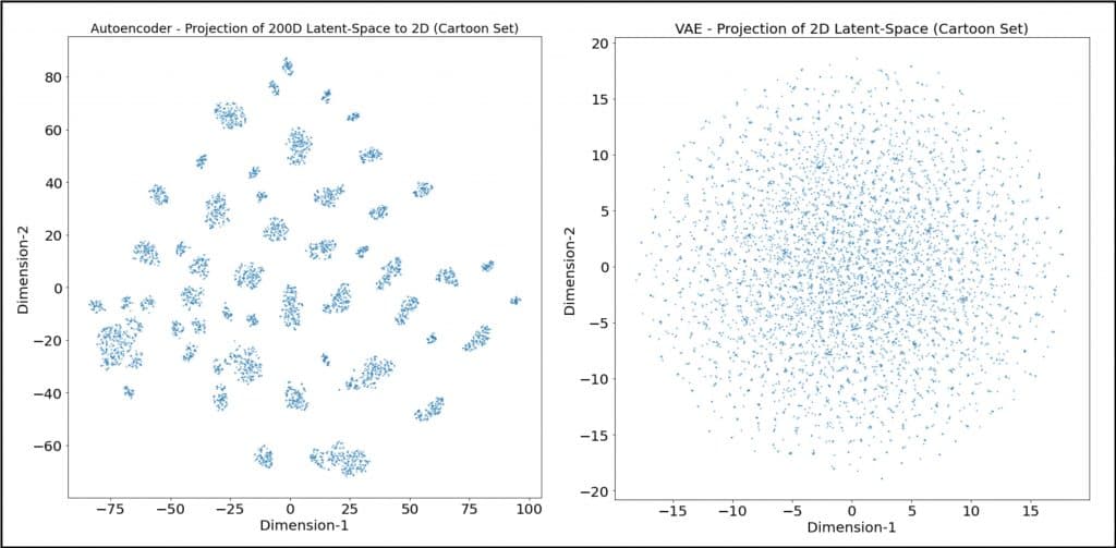
We did a similar experiment with Cartoon Set trained VAE, and from the VAE plot ( on the right ), we can observe that the data points, when projected to latent-space, are continuous, meaning there are no gaps. While the Autoencoder plot ( on the left ) has many gaps, forms various small clusters distant from each other, and the data points seem highly discontinuous.

Also, check the range of the x-axis and y-axis of both the plots; you can clearly see that Autoencoder’s data points are spread across a large interval.

Do check out the tutorial on Introduction to Autoencoder in TensorFlow, where we do extensive, similar experiments.

Reconstructing Images Randomly from Latent Spaces

Reconstructing Fashion Images with Latent-Vector Sampled Uniformly

In this experiment, we will take the lower bound and upper bound from the fashion-mnist latent-space ( two dimensions ) and sample two NumPy arrays, each of size [10, 1] with a uniform distribution. We will concatenate these arrays x and y respectively, and feed it to the decoder. In short, we pick a 2D point ( within the lower & upper bound ) with a uniform distribution from the latent-space and feed it to the decoder.

Finally, we will plot these images.

figsize = 15

min_x = min(embeddings[:, 0])
max_x = max(embeddings[:, 0])
min_y = min(embeddings[:, 1])
max_y = max(embeddings[:, 1])


x = np.random.uniform(min_x,max_x, size = 10)
y = np.random.uniform(min_y,max_y, size = 10)
z_grid = np.array(list(zip(x, y)))
reconst = dec.predict(z_grid)


fig = plt.figure(figsize=(figsize, 10))

for i in range(10):
    ax = fig.add_subplot(5, 5, i+1)
    ax.axis('off')
    ax.text(0.5, -0.15, str(np.round(z_grid[i],1)), fontsize=10, ha='center', transform=ax.transAxes)
    
    ax.imshow(reconst[i, :,:,0]*255, cmap = 'gray')

We can see that the images reconstructed by VAE have a great perceptual quality. Remember we are only using the decoder here and there is no involvement of the encoder and sampling network.

Reconstructing Fashion Images with Latent-Vector Sampled from Normal Distribution

This one is an interesting experiment; recall that we trained our VAE in such a way that the mean and variance latent variables are close to the standard normal distribution, and as a result, the latent vector z sampled from the latent variables follow a normal distribution. By doing so, the decoder learned to generate images of the dataset given a z vector sampled from a normal distribution. And that’s what we do in this experiment.

figsize = 15

x = np.random.normal(size = (10,2))
reconstruct = dec.predict(x)

fig = plt.figure(figsize=(figsize, 10))

for i in range(10):
    ax = fig.add_subplot(5, 5, i+1)
    ax.axis('off')
    ax.imshow(reconstruct[i, :,:,0]*255, cmap = 'gray')

Reconstructing Cartoon Images with Latent-Vector Sampled Uniformly

We do a similar experiment we did for VAE trained with Fashion-MNIST. However, we cannot sample a point uniformly from a latent-space of 200D by simply passing the lower bound and upper bound to np.random.uniform() since we will need to do this for all 200D ( it expects a scalar value ). Instead, we take the minimum and maximum of the 200D across all 5K images, sample a uniform matrix of size [10, 200] whose values lie between [0, 1]. We then scale these values by taking the difference between the minimum and maximum of the latent-space. Finally, we pass the scaled output to the decoder and generate the images.

figsize = 15


min_x = lat_space.min(axis=0)
max_x = lat_space.max(axis=0)
x = np.random.uniform(size = (10,200))
x = x * (max_x - (np.abs(min_x))) 
print(x.shape)
reconstruct = dec.predict(x)


fig = plt.figure(figsize=(figsize, 10))
fig.subplots_adjust(hspace=0.2, wspace=0.2)

for i in range(10):
    ax = fig.add_subplot(5, 5, i+1)
    ax.axis('off')
    pred = reconstruct[i, :, :, :] * 255
    pred = np.array(pred)  
    pred = pred.astype(np.uint8)
    ax.imshow(pred)

As expected, VAE did a great job of generating cartoon images which look similar to the images we have in our dataset.

Reconstructing Cartoon Images from a Latent-Vector Sampled with Normal Distribution

Finally, we perform one last experiment i.e. sampling a vector from a normal distribution and generating images through the decoder.

figsize = 15

x = np.random.normal(size = (10,200))
reconstruct = dec.predict(x)


fig = plt.figure(figsize=(figsize, 10))

for i in range(10):
    ax = fig.add_subplot(5, 5, i+1)
    ax.axis('off')
    pred = reconstruct[i, :, :, :] * 255
    pred = np.array(pred)  
    pred = pred.astype(np.uint8)
    ax.imshow(pred)

And Voila! The decoder of VAE did a fantastic job of generating images similar to the ones in the Cartoon Set.

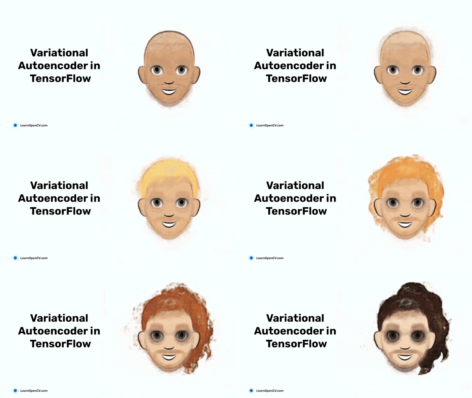
The above-generated images might not be present in the dataset, but they follow a normal distribution. One good example of an image not present in the dataset could be a cartoon face generated by the decoder with a different hairstyle & hair color. In contrast, the same cartoon face might not have the same hairstyle or hair color within the dataset.

Conclusion

Congratulations on making this far; we know it was a lot to take in, so let’s summarize:

We started with Introduction to Variational Autoencoder ( VAE ) and how it overcomes the caveats in vanilla autoencoder.
We discussed the loss function of VAE.
Then we learned about the Reparametrization trick in VAE.
We implemented an autoencoder in TensorFlow on two datasets: Fashion-MNIST and Cartoon Set Data.
We did various experiments like visualizing the latent-space, generating images sampled uniformly from the latent-space, comparing the latent-space of an autoencoder and variational autoencoder.
We generated fashion-mnist and cartoon images with a latent-vector sampled from a normal distribution.

Thank you so much for reading this! Hope by reading this blog post; you got to learn a lot about variational autoencoder. ?

Variational Autoencoder in TensorFlow

Introduction to Variational Autoencoder

VAE Objective

Objective Function of VAE

Reconstruction Error

KL Divergence

Reparameterization Trick

Coding a Variational Autoencoder in TensorFlow

Dataset

Importing Modules

Loading and Preprocessing Dataset

Architectural Diagram of Autoencoder

Define the Encoder Network

The Sampling Network

Define the Decoder Network

Optimizer and Loss Function

Training the Variational Autoencoder

Reconstructing Test Images

Variational Autoencoder with Cartoon Set Data

Dataset

Loading and Preprocessing the Data

Variational Autoencoder Architecture

Define the Encoder Network

The Decoder Network

Reconstructing the Cartoon Images

Visualizing the Latent Space

Latent Space Projection of Variational Autoencoder Trained on Fashion-MNIST

Latent Space Projection with t-SNE of VAE Trained on Cartoon Set

Reconstructing Images Randomly from Latent Spaces

Reconstructing Fashion Images with Latent-Vector Sampled Uniformly

Reconstructing Fashion Images with Latent-Vector Sampled from Normal Distribution

Reconstructing Cartoon Images with Latent-Vector Sampled Uniformly

Reconstructing Cartoon Images from a Latent-Vector Sampled with Normal Distribution

Conclusion

Get Started with OpenCV

Subscribe to receive the download link, receive updates, and be notified of bug fixes

Which email should I send you the download link?

Introduction to Variational Autoencoder

VAE Objective

Objective Function of VAE

Reconstruction Error

KL Divergence

Reparameterization Trick

Coding a Variational Autoencoder in TensorFlow

Dataset

Importing Modules

Loading and Preprocessing Dataset

Architectural Diagram of Autoencoder

Define the Encoder Network

The Sampling Network

Define the Decoder Network

Optimizer and Loss Function

Training the Variational Autoencoder

Reconstructing Test Images

Variational Autoencoder with Cartoon Set Data

Dataset

Loading and Preprocessing the Data

Variational Autoencoder Architecture

Define the Encoder Network

The Decoder Network

Reconstructing the Cartoon Images

Visualizing the Latent Space

Latent Space Projection of Variational Autoencoder Trained on Fashion-MNIST

Latent Space Projection with t-SNE of VAE Trained on Cartoon Set

Reconstructing Images Randomly from Latent Spaces

Reconstructing Fashion Images with Latent-Vector Sampled Uniformly

Reconstructing Fashion Images with Latent-Vector Sampled from Normal Distribution

Reconstructing Cartoon Images with Latent-Vector Sampled Uniformly

Reconstructing Cartoon Images from a Latent-Vector Sampled with Normal Distribution

Conclusion

Subscribe & Download Code

Get Started with OpenCV

Subscribe to receive the download link, receive updates, and be notified of bug fixes

Which email should I send you the download link?