Diffusion models have changed the game in image generation. Tools like Stable Diffusion have become popular for their ability to turn text into images using these models. The core idea behind diffusion models, including DDPM (Denoising Diffusion Probabilistic Models), is that noise is gradually added to an image, and then the model learns how to reverse that noise. However, this process can be slow, which leads to longer generation times. Enter DDIM (Denoising Diffusion Implicit Models), a faster alternative that accelerates the process without sacrificing quality.
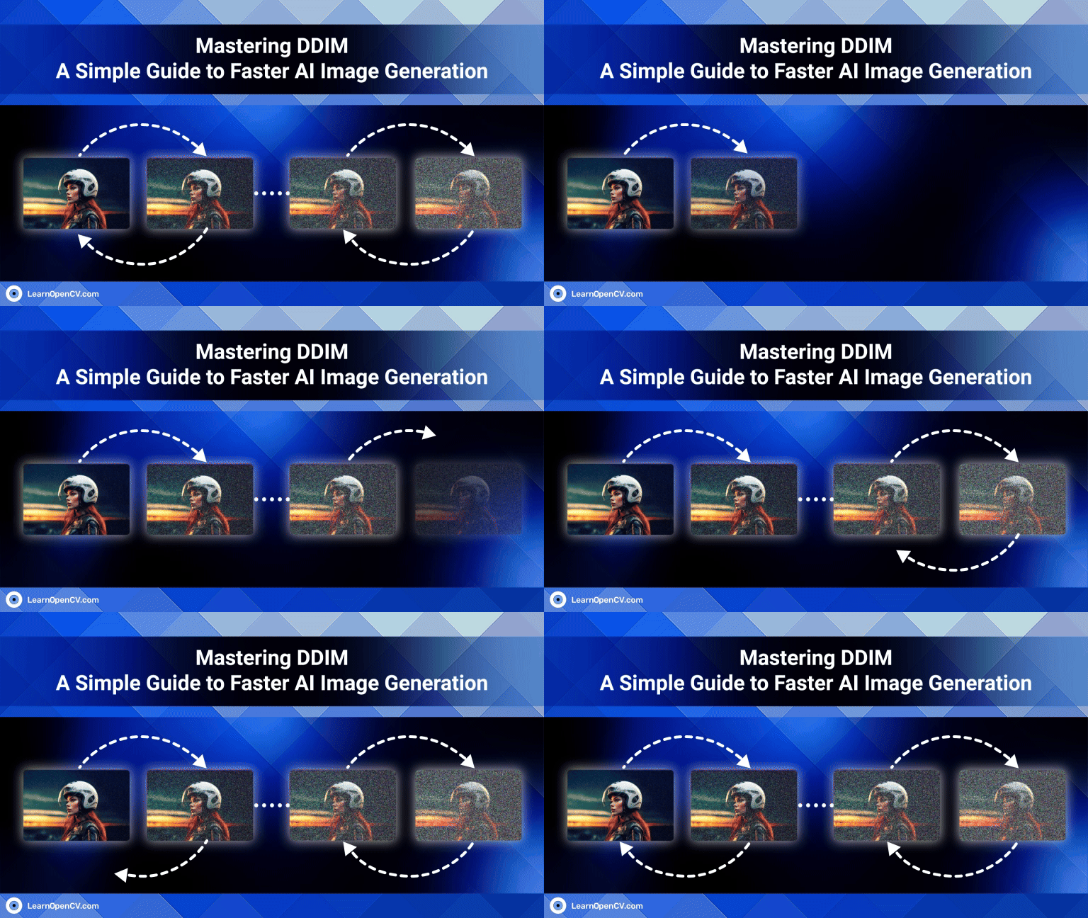
A faster alternative, DDIM, evolved from the original DDPM (Denoising Diffusion Probabilistic Models). While DDPM was groundbreaking, DDIM brought improvements by making the reverse process deterministic.
In this article, we’ll walk through a theoretical understanding of DDIMs, explore key improvements over DDPM, and guide you through using DDIM with simple code examples.
- What is a Diffusion model?
- Why are DDPMs so slow?
- What is DDIM?
- DDIM vs DDPM: What’s the Difference?
- The Mathematical Section: From DDPMs to DDIMs
- DDIM in Code (Using HuggingFace Diffusers)
- Can DDIM Work with Other Diffusion Models?
- Real-World Applications of DDIM
- Bonus: DDIM Also Enables Style Variation
- Summary
- Final Thoughts
- 🔗 References
What is a Diffusion model?
Before covering DDIM, let’s first understand what Denoising Diffusion Probabilistic models or DDPMs are.
A diffusion model works in two steps:
- The Forward process: Gradually adding noise
The forward process in a diffusion model starts with an initial image, typically a high-quality, clean image, which is then corrupted over time by the repetitive addition of noise. This sequence of transformations continues until the image is entirely converted into random noise.- The mathematical formulation of this process is represented by:

- Where,
 represents the image at timestep
  ,
, controls how much noise is added at each step,
 governs the noise level at each stage.
- The mathematical formulation of this process is represented by:

- The Reverse process: recovering the original image
The goal of the reverse process is to denoise the noisy image at each step and recover the original image. During the reverse process, the model utilizes the learned probability distributions to predict and remove the noise at each timestep. The reverse process is not purely deterministic; it involves some stochasticity that allows for randomness in generating new images. This stochastic nature ensures diversity in the generated outputs.- Mathematically, it is represented as:

- Where,
 is the predicted mean of the original image at timestep
  ,
, represents the variance, which models the uncertainty at each step.
- Mathematically, it is represented as:
Here’s a toy example in code using PyTorch:
import torch
import torch.nn.functional as F

## X_0 represents the final target image, X_T represents complete noise

# defining how should noise be added to the image in gradual timesteps
def linear_beta_schedule(timesteps, start = 0.001, end = 0.02):
    return torch.linspace(start, end, timesteps)

#
def get_index_from_list(vals, t, x_shape):
    batch_size = t.shape[0]
    output = vals.gather(-1, t.cpu())
    return output.reshape(batch_size, *((1,) * (len(x_shape) - 1))).to(t.device)

def noise_scheduler(x_0, t, sqrt_alphas_cumprod, sqrt_one_minus_alphas_cumprod, device = "cpu"):
    x_0 = x_0.float()
    noise = torch.randn_like(x_0)           # random numbers from a normal distribution with mean 0 and variance 1
    sqrt_alphas_cumprod_t = get_index_from_list(sqrt_alphas_cumprod, t, x_0.shape)
    sqrt_one_minus_alphas_cumprod_t = get_index_from_list( sqrt_one_minus_alphas_cumprod, t, x_0.shape)

    # mean( square_root_alpha * x_0 ) + variance( one_minus_square_root_alpha * epsilon )
    return sqrt_alphas_cumprod_t.to(device)*x_0.to(device) + sqrt_one_minus_alphas_cumprod_t.to(device) * noise.to(device), noise.to(device)
Why are DDPMs so slow?
The reverse process in traditional diffusion models (like DDPM) involves hundreds or thousands of steps. The larger the number of timesteps, the more passes the image must go through the neural network, resulting in an increased computational load.

For example:
- DDPM (Denoising Diffusion Probabilistic Model) typically requires 1000 steps to generate a single image.
- Even with optimizations such as reducing the number of time steps, the model still requires at least hundreds of steps to generate an image of acceptable quality.
Difficulties in low-latency environment
The computational cost of DDPMs makes them unsuitable for specific applications that require real-time or high-speed image generation. For instance, in environments where low latency is crucial—such as interactive art generation or on-demand image synthesis—DDPMs can struggle to meet performance requirements. The high number of timesteps and extensive computational demands make it challenging to deploy DDPMs in real-world applications where quick results are needed.
What is DDIM?
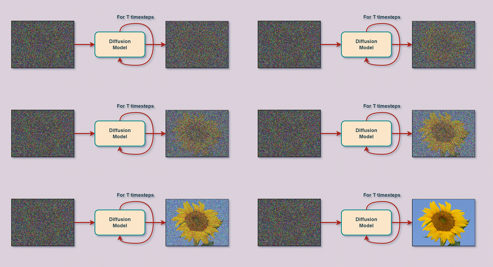
DDIM (Denoising Diffusion Implicit Models) was introduced in 2021 by researchers Jiaming Song, Chenlin Meng, and Stefano Ermon to improve earlier diffusion models, especially DDPM (Denoising Diffusion Probabilistic Models). The main goal of DDIM was simple: to speed up the process of creating images using diffusion models.
DDIM removes the noise clearly and predictably (called a deterministic process). Because of this change, DDIM can generate great-looking images in much fewer steps—often around 50 to 100 steps instead of the typical 1000.
Plus, you don’t need to retrain the model if you’re already using diffusion models—DDIM can work right away.
Key Features of DDIM
- Much faster sampling (e.g., only 50 steps instead of 1000)
- Deterministic reverse process
- Compatible with pre-trained diffusion models
- Maintains high image quality
DDIM vs DDPM: What’s the Difference?
Let’s break it down simply:
| Feature | DDPM | DDIM |
| Reverse Process | Stochastic (random noise) | Deterministic (no random noise) |
| Sampling Speed | Slow (up to 1000 steps) | Fast (as low as 50 steps) |
| Image Quality | Very High | Almost the same |
| Retraining Needed? | Yes, if you change steps | No, use same model |
DDIMs maintain high sample quality even with significantly fewer sampling steps. On CIFAR-10, DDIMs achieve comparable FID scores to DDPMs while requiring only 10-20 steps instead of 1000, representing a 50- 100x speedup.

The Mathematical Section: From DDPMs to DDIMs
DDIMs introduce a critical innovation by generalizing the forward process to a non-Markovian process while maintaining the same training objective as DDPMs.

When the parameter ![]() is set to zero (
is set to zero (![]() ), the forward diffusion process becomes fully deterministic. In simpler terms, each step becomes predictable, mapping clean images directly to noisy versions without randomness. This leads to what’s known as an implicit probabilistic model, where there’s a precise, fixed mapping between the initial noise and the generated final images.
), the forward diffusion process becomes fully deterministic. In simpler terms, each step becomes predictable, mapping clean images directly to noisy versions without randomness. This leads to what’s known as an implicit probabilistic model, where there’s a precise, fixed mapping between the initial noise and the generated final images.
The deterministic DDIM sampling process is expressed mathematically as:
![]()
where ![]() are the predicted noise.
are the predicted noise.
DDIM in Code (Using Hugging Face Diffusers)
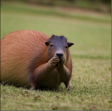
Let’s try out DDIM with an accurate image-generation pipeline. We’ll use HuggingFace’s diffusers library, which makes working with DDIM very easy.
!pip install -U diffusers
!pip install transformers
!pip install accelerate
!pip install sentencepiece
!pip install protobuf
The given code will work only after logging into hugging face using your personal access token. The below image displays the command and how would the terminal output will look like.

import torch
from diffusers import StableDiffusionPipeline, DDIMScheduler
import matplotlib.pyplot as plt

pipe = StableDiffusionPipeline.from_pretrained("CompVis/stable-diffusion-v1-4", torch_dtype = torch.float16, safety_checker = None)
pipe.scheduler = DDIMScheduler.from_config(
    pipe.scheduler.config
)
pipe.to("cuda")

torch.manual_seed(1283012) #any random 6 or 7 digit seed will be good

image = pipe("a cute capybara").images[0]
plt.imshow(image)
plt.show()
Can DDIM Work with Other Diffusion Models?
Absolutely. One significant advantage of DDIM is its compatibility and flexibility with various diffusion-based generative models. DDIM isn’t restricted to a single architecture or specific diffusion model. Instead, it leverages the exact noise prediction mechanism already learned by models like:
- Stable Diffusion
- Imagen
- OpenAI’s Diffusion Models
This means you can easily integrate DDIM into existing diffusion pipelines. By simply changing the sampling method, DDIM allows these pre-trained models to generate images more rapidly without requiring extensive retraining or adjustments.
Real-World Applications of DDIM
DDIM’s deterministic and accelerated sampling capability makes it particularly suitable for applications where speed, consistency, and efficiency matter. Here are some areas where DDIM excels:
1. Rapid Image Generation
Creative professionals, including graphic designers, digital artists, and concept artists, often need to quickly generate multiple image concepts. DDIM accelerates this process dramatically, enabling faster iterations and more efficient workflows.
2. Real-time AI Image Applications
Applications like AI-powered art generators (e.g., Lensa, Dream) significantly benefit from DDIM’s speed. Faster image generation means quicker results and enhanced user experiences, particularly in mobile and web-based environments where responsiveness is critical.

3. Research and Prototyping
Researchers and developers exploring generative models often require extensive experimentation. DDIM allows rapid prototyping by reducing the waiting time associated with conventional diffusion models, enabling quicker validation of ideas and accelerating the development cycle.
Bonus: DDIM Also Enables Style Variation
Another benefit of DDIM’s deterministic sampling process is its capability to control stylistic variations systematically. By slightly modifying initial noise conditions or adjusting parameters like “eta” (which introduces controlled randomness), you can produce diverse yet consistent variations of an image:
pipe.scheduler.eta = 0.3  # Add some controlled randomness
image = pipe(prompt, num_inference_steps=50).images[0]
This feature is particularly valuable for:
- Generating consistent image variations
- Creating smooth and coherent animation frames
- Enabling controlled creative exploration
Summary
Here’s everything we covered:
- DDIM is a faster alternative to DDPM for image generation
- Uses a deterministic reverse process, reducing randomness
- Supports fewer steps without hurting quality much
- Works with existing pre-trained models
- Easy to implement with Hugging Face
diffusers
Final Thoughts
DDIM significantly accelerates image generation compared to DDPM by adopting a deterministic approach, making diffusion models accessible and efficient for real-world applications.
Interestingly, while earlier versions of Stable Diffusion commonly employed the DDIM scheduler, the more recent Stable Diffusion 3.5 utilizes a different scheduler called FlowMatchEulerDiscreteScheduler.
Unlike DDIM’s deterministic denoising, FlowMatchEulerDiscreteScheduler leverages advanced numerical integration techniques inspired by flow-based generative models, offering improved image coherence, sharper details, and even faster generation times in some scenarios.
Nevertheless, DDIM remains highly valuable due to its simplicity, widespread compatibility, and proven reliability, especially when predictable outcomes and straightforward implementation are prioritized.
🔗 References
- DDIM: Denoising Diffusion Implicit Models (arXiv)
- Hugging Face Diffusers Documentation
- Stable Diffusion v1.4 on Hugging Face
- Lucidrains’ Denoising Diffusion Models (GitHub)
- Thanks to Ollin Boer Bohan for providing an incredible resource on Diffusion Models







100K+ Learners
Join Free OpenCV Bootcamp3 Hours of Learning