


Billionaire investor and entrepreneur Peter Thiel’s favorite contrarian questions is
What important truth do very few people agree with you on?
If you had asked this question to Prof. Geoffrey Hinton in the year 2010, he would have answered that Convolutional Neural Networks (CNN) had the potential to produce a seismic shift in solving the problem of image classification. Back then researchers in the field would not have bothered to think twice about that comment. Deep Learning was that uncool!
That was the year ImageNet Large Scale Visual Recognition Challenge (ILSVRC) was launched.
In two years, with the publication of the paper, “ImageNet Classification with Deep Convolutional Neural Networks” by Alex Krizhevsky, Ilya Sutskever, and Geoffrey E. Hinton, he and a handful of researchers were proven right. It was a seismic shift that broke the Richter scale! The paper forged a new landscape in Computer Vision by demolishing old ideas in one masterful stroke.
The paper used a CNN to get a Top-5 error rate (rate of not finding the true label of a given image among its top 5 predictions) of 15.3%. The next best result trailed far behind (26.2%). When the dust settled, Deep Learning was cool again.
In the next few years, multiple teams would build CNN architectures that beat human level accuracy.
The architecture used in the 2012 paper is popularly called AlexNet after the first author Alex Krizhevsky. In this post, we will go over its architecture and discuss its key contributions.
Input
As mentioned above, AlexNet was the winning entry in ILSVRC 2012. It solves the problem of image classification where the input is an image of one of 1000 different classes (e.g. cats, dogs etc.) and the output is a vector of 1000 numbers. The ith element of the output vector is interpreted as the probability that the input image belongs to the ith class. Therefore, the sum of all elements of the output vector is 1.
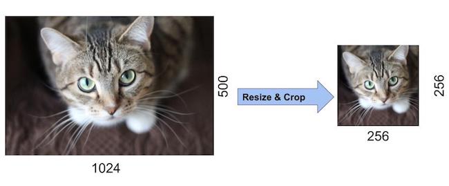
The input to AlexNet is an RGB image of size 256×256. This means all images in the training set and all test images need to be of size 256×256.
If the input image is not 256×256, it needs to be converted to 256×256 before using it for training the network. To achieve this, the smaller dimension is resized to 256 and then the resulting image is cropped to obtain a 256×256 image. The figure below shows an example.
If the input image is grayscale, it is converted to an RGB image by replicating the single channel to obtain a 3-channel RGB image. Random crops of size 227×227 were generated from inside the 256×256 images to feed the first layer of AlexNet. Note that the paper mentions the network inputs to be 224×224, but that is a mistake and the numbers make sense with 227×227 instead.


AlexNet Architecture
AlexNet was much larger than previous CNNs used for computer vision tasks ( e.g. Yann LeCun’s LeNet paper in 1998). It has 60 million parameters and 650,000 neurons and took five to six days to train on two GTX 580 3GB GPUs. Today there are much more complex CNNs that can run on faster GPUs very efficiently even on very large datasets. But back in 2012, this was huge!
Let’s look at the architecture. You can click on the image below to enlarge it.

AlexNet consists of 5 Convolutional Layers and 3 Fully Connected Layers.
Multiple Convolutional Kernels (a.k.a filters) extract interesting features in an image. In a single convolutional layer, there are usually many kernels of the same size. For example, the first Conv Layer of AlexNet contains 96 kernels of size 11x11x3. Note the width and height of the kernel are usually the same and the depth is the same as the number of channels.
The first two Convolutional layers are followed by the Overlapping Max Pooling layers that we describe next. The third, fourth and fifth convolutional layers are connected directly. The fifth convolutional layer is followed by an Overlapping Max Pooling layer, the output of which goes into a series of two fully connected layers. The second fully connected layer feeds into a softmax classifier with 1000 class labels.
ReLU nonlinearity is applied after all the convolution and fully connected layers. The ReLU nonlinearity of the first and second convolution layers are followed by a local normalization step before doing pooling. But researchers later didn’t find normalization very useful. So we will not go in detail over that.
Overlapping Max Pooling
Max Pooling layers are usually used to downsample the width and height of the tensors, keeping the depth same. Overlapping Max Pool layers are similar to the Max Pool layers, except the adjacent windows over which the max is computed overlap each other. The authors used pooling windows of size 3×3 with a stride of 2 between the adjacent windows. This overlapping nature of pooling helped reduce the top-1 error rate by 0.4% and top-5 error rate by 0.3% respectively when compared to using non-overlapping pooling windows of size 2×2 with a stride of 2 that would give same output dimensions.
ReLU Nonlinearity

An important feature of the AlexNet is the use of ReLU(Rectified Linear Unit) Nonlinearity. Tanh or sigmoid activation functions used to be the usual way to train a neural network model. AlexNet showed that using ReLU nonlinearity, deep CNNs could be trained much faster than using the saturating activation functions like tanh or sigmoid. The figure below from the paper shows that using ReLUs(solid curve), AlexNet could achieve a 25% training error rate six times faster than an equivalent network using tanh(dotted curve). This was tested on the CIFAR-10 dataset.
Lets see why it trains faster with the ReLUs. The ReLU function is given by
f(x) = max(0,x)
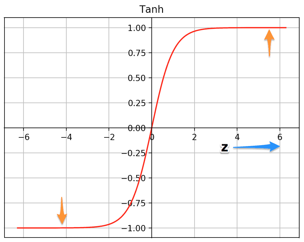

Above are the plots of the two functions – tanh and ReLU. The tanh function saturates at very high or very low values of z. At these regions, the slope of the function goes very close to zero. This can slow down gradient descent. On the other hand the ReLU function’s slope is not close to zero for higher positive values of z. This helps the optimization to converge faster. For negative values of z, the slope is still zero, but most of the neurons in a neural network usually end up having positive values. ReLU wins over the sigmoid function too for the same reason.
Reducing Overfitting
What is overfitting?
Remember the kid from your middle school class who did very well in tests, but did poorly whenever the questions on the test required original thinking and were not covered in the class? Why did he do so poorly when confronted with a problem he had never seen before? Because he had memorized the answers to questions covered in the class without understanding the underlying concepts.
Similarly, the size of the Neural Network is its capacity to learn, but if you are not careful, it will try to memorize the examples in the training data without understanding the concept. As a result, the Neural Network will work exceptionally well on the training data, but they fail to learn the real concept. It will fail to work well on new and unseen test data. This is called overfitting.
The authors of AlexNet reduced overfitting using a couple of different methods.
Data Augmentation
Showing a Neural Net different variation of the same image helps prevent overfitting. You are forcing it to not memorize! Often it is possible to generate additional data from existing data for free! Here are few tricks used by the AlexNet team.
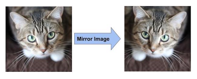
Data Augmentation by Mirroring
If we have an image of a cat in our training set, its mirror image is also a valid image of a cat. Please see the figure below for an example. So we can double the size of the training dataset by simply flipping the image about the vertical axis.
Data Augmentation by Random Crops
In addition, cropping the original image randomly will also lead to additional data that is just a shifted version of the original data.
The authors of AlexNet extracted random crops of size 227×227 from inside the 256×256 image boundary to use as the network’s inputs. They increased the size of the data by a factor of 2048 using this method.

Notice the four randomly cropped images look very similar but they are not exactly the same. This teaches the Neural Network that minor shifting of pixels does not change the fact that the image is still that of a cat. Without data augmentation, the authors would not have been able to use such a large network because it would have suffered from substantial overfitting.
Dropout
With about 60M parameters to train, the authors experimented with other ways to reduce overfitting too. So they applied another technique called dropout that was introduced by G.E. Hinton in another paper in 2012. In dropout, a neuron is dropped from the network with a probability of 0.5. When a neuron is dropped, it does not contribute to either forward or backward propagation. So every input goes through a different network architecture, as shown in the animation below. As a result, the learnt weight parameters are more robust and do not get overfitted easily. During testing, there is no dropout and the whole network is used, but output is scaled by a factor of 0.5 to account for the missed neurons while training. Dropout increases the number of iterations needed to converge by a factor of 2, but without dropout, AlexNet would overfit substantially.
Today dropout regularization is very important and implementations that are better than the original one have been developed. We will focus and go over Dropout Regularization alone in a future post.
References:
ImageNet Classification with Deep Convolutional Neural Networks by Alex Krizhevsky, Ilya Sutskever, and Geoffrey E. Hinton, 2012
Coursera course on “Convolutional Neural Network” as part of the Deep Learning Specialization by Andrew Ng.