YOLOv3 is one of the most popular real-time object detectors in Computer Vision.
In our previous post, we shared how to use YOLOv3 in an OpenCV application. It was very well received, and many readers asked us to write a post on training YOLOv3 for new objects (i.e. custom data).
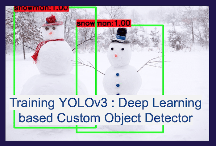
In this step-by-step tutorial, we start with a simple case of how to train a 1-class object detector using YOLOv3. The training YOLOv3 tutorial is written with beginners in mind. Continuing with the spirit of the holidays, we will build our own snowman detector.
In this post, we will share the training process, scripts helpful in training, and results of some publicly available snowman images and videos. You can use the same procedure to train an object detector with multiple objects.
YOLO Master Post – Every Model Explained
Unlock the full story behind all the YOLO models’ evolutionary journey: Dive into our extensive pillar post, where we unravel the evolution from YOLOv1 to YOLO-NAS. This essential guide is packed with insights, comparisons, and a deeper understanding that you won’t find anywhere else.
Don’t miss out on this comprehensive resource — Mastering All Yolo Models for a richer, more informed perspective on the YOLO series.
1. Dataset
As with any deep learning task, the first most important task is to prepare the dataset. We will use the snowman images from Google’s OpenImagesV4 dataset, which is publicly available online. It is a huge dataset with around 600 different classes of object. The dataset also contains the bounding box annotations for these objects. As a whole, the dataset is more than 500GB, but we will download the images with ‘Snowman’ objects only. Copyright Notice
We do not own the copyright to these images, and therefore we are following the standard practice of sharing sources to the images and not the image files themselves. OpenImages has the originalURL and license information for each image. Any use of this data (academic, non-commercial, or commercial) is at your own legal risk.
1.1 Download data [approx 1 hour]
First, we will need to install awscli
sudo pip3 install awscli
Then we need to get the relevant
wget https://storage.googleapis.com/openimages/2018_04/class-descriptions-boxable.csv

wget https://storage.googleapis.com/openimages/2018_04/train/train-annotations-bbox.csv
Next, move the above .csv files to the same folder as the downloaded code and then use the following script to download the data.
python3 getDataFromOpenImages_snowman.py
The images get downloaded into the JPEGImages folder, and the corresponding label files are written into the labels folder. The download will get 770 snowman instances on 539 images. The download can take around an hour, which can vary depending on internet speed. Both the JPEGImages and labels together should be less than 136 MB.
For multiclass object detectors, where you will need more samples for each class, you might want to get the test-annotations-bbox.csv and validation-annotations-bbox.csv files, too, and then modify runMode in the python script and rerun it to get more images for each class. But in our current snowman case, 770 instances are sufficient.
1.3 Train-test split
Any machine learning training procedure involves first splitting the data randomly into two sets.
- Training set: This is the part of the data on which we are training the Yolov3 model. Depending on the amount of data you have, you can randomly select between 70% to 90% of the data for training.
- Test set: This is the part of the data on which we test our model. Typically, this is 10-30% of the data. No image should be part of both the training and the test set.
We split the images inside the JPEGImages folder into the train and test sets. You can do it using the splitTrainAndTest.py scripts as follows, passing on the full path of the JPEGImages folder as an argument.
python3 splitTrainAndTest.py /full/path/to/snowman/JPEGImages/
The above script splits the data into a train (90%) and a test set (10%) and generates two files snowman_train.txt and snowman_test.txt
2. Darknet
In this tutorial, we use Darknet by Joseph Redmon. It is a deep-learning framework written in C.
2.1 Download and build Darknet
Let’s first download and build it on your system.
cd ~
git clone https://github.com/pjreddie/darknet
cd darknet
make
2.2 Modify code to save model files regularly
After we make sure the original repo compiles in your system, let’s make some minor modifications in order to store the intermediate weights. In the file examples/detector.c, change line#135 from
if(i%10000==0 || (i < 1000 && i%100 == 0)){
to
if(i%1000==0 || (i < 2000 && i%200 == 0)){
The original repo saves the network weights after every 100 iterations till the first 1000 and then saves only after every 10000 iterations. In our case, since we are training with only a single class, we expect our training to converge much faster. So to monitor the progress closely, we save after every 200 iterations till we reach 2000, and then we save after every 1000 iterations. After the above changes are made, recompile darknet using the make command again.
We ran the experiments using an NVIDIA GeForce GTX 1080 GPU. Let’s now get into some more details required to run the training successfully.
3. Data Annotation
We have shared the label files with annotations in the labels folder. Each row entry in a label file represents a single bounding box in the image and contains the following information about the box:
<object-class-id> <center-x> <center-y> <width> <height>
The first field object-class-id is an integer representing the class of the object. It ranges from 0 to (number of classes – 1). In our current case, since we have only one class of snowman, it is always set to 0.
The second and third entry, center-x and center-y are respectively the x and y coordinates of the center of the bounding box, normalized (divided) by the image width and height, respectively.
The fourth and fifth entry, width and height are respectively the width and height of the bounding box, again normalized (divided) by the image width and height, respectively.
Let’s consider an example with the following notations:
$x$ – x-coordinate(in pixels) of the center of the bounding box
$y$ – y-coordinate(in pixels) of the center of the bounding box
$w$ – width(in pixels) of the bounding box
$h$ – height(in pixels) of the bounding box
$W$ – width(in pixels) of the whole image
$H$ – height(in pixels) of the whole image
Then we compute the annotation values in the label files as follows:
center-x = $x / W$
center-y = $y / H$
width = $w / W$
height = $h / H$
The above four entries are all floating point values between 0 to 1.
4. Download the Pre-trained model
When you train your own object detector, it is a good idea to leverage existing models trained on extensive datasets, even though the large dataset may not contain the object you are trying to detect. This process is called transfer learning.
Instead of learning from scratch, we use a pre-trained model which contains convolutional weights trained on ImageNet. Using these weights as our starting weights, our network can learn faster. Let’s download it now to our darknet folder.
cd ~/darknet
wget https://pjreddie.com/media/files/darknet53.conv.74 -O ~/darknet/darknet53.conv.74
5. Data file
In the file darknet.data(included in our code distribution), we need to provide information about the specifications for our object detector and some relevant paths.
classes = 1
train  = /path/to/snowman/snowman_train.txt
valid  = /path/to/snowman/snowman_test.txt
names = /path/to/snowman/classes.names
backup = /path/to/snowman/weights/
The classes parameter needs the number of classes. In our case, it is 1.
You need to provide the absolute paths of the files snowman_train.txt and snowman_test.txt generated earlier, which have the list of files to be used for training(train parameter) and validation(valid parameter) respectively.
The names field represents the path of a file that contains the names of all the classes. We have included the classes.names file, which contains the class name ‘snowman’. You will need to provide its absolute path in your machine here.
Lastly, for the backup parameter, we need to give the path to an existing directory to store the intermediate weights files as the training progresses.
6. YOLOv3 configuration parameters
Along with the darknet.data and classes.names files, YOLOv3 also needs a configuration file darknet-yolov3.cfg. It is also included in our code base. It is based on the demo configuration file, yolov3-voc.cfg (comes with darknet code), which was used to train on the VOC dataset. All the important training parameters are stored in this configuration file. Let us understand what they mean and what values to set them to.
6.1 Batch hyper-parameter in training YOLOv3
Let’s learn more about batch and subdivision parameter.
# Testing
# batch=1
# subdivisions=1
# Training
batch=64
subdivisions=16
The batch parameter indicates the batch size used during training.
Our training set contains a few hundred images, but it is not uncommon to train on millions of images. The training process involves iteratively updating the weights of the neural network based on how many mistakes it is making on the training dataset.
It is impractical (and unnecessary) to use all images in training the set at once to update the weights. So, a small subset of images is used in one iteration, and this subset is called the batch size.
When the batch size is set to 64, it means 64 images are used in one iteration to update the parameters of the neural network.
6.2 Subdivisions configuration parameter in training YOLOv3
Even though you may want to use a batch size of 64 for training your neural network, you may not have a GPU with enough memory to use a batch size of 64. Fortunately, Darknet allows you to specify a variable called subdivisions that lets you process a fraction of the batch size at one time on your GPU.
You can start the training with subdivisions=1, and if you get an Out of memory error, increase the subdivision parameter by multiples of 2(e.g. 2, 4, 8, 16) till the training proceeds successfully. The GPU will process $batch/subdivision$ number of images at any time, but the full batch or iteration would be complete only after all the 64 (as set above) images are processed.
During testing, both batch and subdivision are set to 1.
6.3 Width, Height, Channels
These configuration parameters specify the input image size and the number of channels.
width=416
height=416
channels=3
The input training images are first resized to width x height before training. Here we use the default values of 416×416. The results might improve if we increase it to 608×608, but it would take longer to train too. channels=3 indicates that we would be processing 3-channel RGB input images.
6.4 Momentum and Decay
The configuration file contains a few parameters that control how the weight is updated.
momentum=0.9
decay=0.0005
In the previous section, we mentioned how the weights of a neural network are updated based on a small batch of images and not the entire dataset. Because of this reason, the weight updates fluctuate quite a bit. That is why a parameter momentum is used to penalize large weight changes between iterations.
A typical neural network has millions of weights, and therefore it can easily overfit any training data. Overfitting simply means it will do very well on training data and poorly on test data. It is almost like the neural network has memorized the answer to all images in the training set but really not learned the underlying concept. One of the ways to mitigate this problem is to penalize large values for weights. The parameter decay controls this penalty term. The default value works just fine, but you may want to tweak this if you notice overfitting.
6.5 Learning Rate, Steps, Scales, Burn In (warm-up)
learning_rate=0.001
policy=steps
steps=3800
scales=.1
burn_in=400
The parameter learning rate controls how aggressively we should learn based on the current batch of data. Typically this is a number between 0.01 and 0.0001.
At the beginning of the training process, we start with zero information and so the learning rate needs to be high. But as the neural network sees a lot of data, the weights need to change less aggressively. In other words, the learning rate needs to be decreased over time. In the configuration file, this decrease in learning rate is accomplished by first specifying that our learning rate decreasing policy is steps. In the above example, the learning rate will start from 0.001 and remain constant for 3800 iterations, and then it will multiply by scales to get the new learning rate. We could have also specified multiple steps and scales.
In the previous paragraph, we mentioned that the learning rate needs to be high initially and low later on. While that statement is largely true, it has been empirically found that the training speed tends to increase if we have a lower learning rate for a short period of time at the very beginning. This is controlled by the burn_in parameter. Sometimes this burn-in period is also called warm-up period.
6.6 Data augmentation
We know data collection takes a long time. For this blog post, we first had to collect 1000 images and then manually create bounding boxes around each of them. It took a team of 5 data collectors 1 day to complete the process.
We want to maximize this data by cooking up new data. This process is called data augmentation. For example, an image of the snowman rotated by 5 degrees is still an image of a snowman. The angle parameter in the configuration file allows you to randomly rotate the given image by ± angle.
Similarly, if we transform the colors of the entire picture using saturation, exposure, and hue, it is still a picture of the snowman.
angle=0
saturation = 1.5
exposure = 1.5
hue=.1
We used the default values for training.
6.7 Number of iterations
Finally, we need to specify how many iterations should the training process be run for.
max_batches=5200
For multi-class object detectors, the max_batches number is higher, i.e. we need to run for more number of batches(e.g. in yolov3-voc.cfg). For an n-classes object detector, it is advisable to run the training for at least 2000*n batches. In our case with only 1 class, 5200 seemed like a safe number for max_batches.
7. Training YOLOv3
Now that we know what all the different components are needed for training let’s start the training process. Go to the darknet directory and start it using the command as following:
cd ~/darknet
./darknet detector train /path/to/snowman/darknet.data /path/to/snowman/darknet-yolov3.cfg ./darknet53.conv.74 > /path/to/snowman/train.log
Make sure you give the correct paths to darknet.data and darknet-yolov3.cfg files in your system. Let’s also save the training log to a file called train.log in your dataset directory so that we can progress the loss as the training goes on.
A useful way to monitor the loss while training is using the grep command on the train.log file
grep "avg" /path/to/snowman/train.log
It shows the batch number, loss in the current batch, average loss till the current batch, current learning rate, time taken for the batch and images used till current batch. As you can see below, the number of images used till each batch increases by an increment of 64. That is because we set the batch size to 64.


As we can see the learning rate increases gradually from 0 to 0.001 by the 400th batch. It would stay there till the 3800th batch when it would again change to 0.0001.
7.1 When do we stop the training?
As the training goes on, the log file contains the loss in each batch. One could argue to stop training after the loss has reached below some threshold. Below is the loss plotted against the batch number for our snowman detector. We generate the plot using the following script:
python3 plotTrainLoss.py /full/path/to/train.log
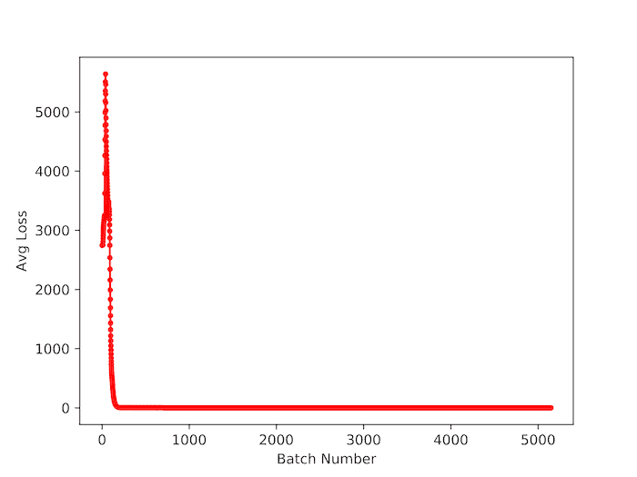
But the actual test should be seeing the mAP using the learned weights. The original darknet code does not have a code to compute mAP. We are working on providing code to compute mAP directly in the darknet code so that you can monitor the precision and recall along with mAP when the weights files are saved. It would come up as a follow-up post. In the meanwhile, you might want to check out AlexAB‘s fork of darknet for computing mAP.
For the snowman detector, we have only 5200 iterations in the configuration file. So you might just let it run till the end. Our final trained weights file, darknet-yolov3_final.weights got a mean Average Precision(mAP) of 70.37%. You can download it here.
8. Testing the model
Along with the loss and mAP, we should always test our weights file on new data and see the results visually to ensure we are happy with the results. In our earlier post, we described how to test the YOLOv3 model using OpenCV. We have included the code for testing your snowman detector. You will need to give the correct path to the modelConfiguration and modelWeights files in object_detection_yolo.py and test with an image or video for snowman detection, e.g.
python3 object_detection_yolo.py --image=snowmanImage.jpg
References:
YOLOv3: An Incremental Improvement
Images displayed in the video were obtained from [1], [2], [3], [4], [5], [6], [7], [8], [9]

