
The recent trend in developing larger and larger Deep Learning models for a slight increase in accuracy raises concerns about their computational efficiency and wide scaled usability. We can not use such huge models on resource-constrained devices like mobiles and embedded devices. Does it mean such devices have to sacrifice accuracy at the cost of a smaller model? Is it possible to deploy these models on devices such as smartphones, a Raspberry Pi, or even on Microcontrollers?
Optimizing the models using TensorFlow Lite is the answer to these questions. This article will introduce the TFLite model in a comprehensive manner. You will learn various supported model optimizations and analyze the performance of the optimized model on an edge device. This blog post is the first in the TensorFlow Lite series.
This blog is the first in the TensorFlow Lite series with the following posts:
- TensorFlow Lite: Model Optimization for On-Device Machine Learning
- TensorFlow Lite Model Maker: Create Models for On-Device Machine Learning
- Deep Dive into TensorFlow Model Optimization Toolkit
- TensorFlow Lite
- Advantages of TensorFlow Lite
- Converting TensorFlow Model to TensorFlow Lite Model
- Base Model Training
- Post Training Quantization using TF Lite
- Performance Evaluation of TF Lite Models on Raspberry Pi
1. TensorFlow Lite – The Tflite Model
TensorFlow Lite (abbr. TF Lite) is an open-source, cross-platform framework that provides on-device machine learning by enabling the models to run on mobile, embedded, and IoT devices.
There are two ways to generate TensorFlow Lite models:
- Converting a TensorFlow model into a TensorFlow Lite model.
- Creating a TensorFlow Lite model from scratch.
We will focus primarily on converting a TensorFlow model into a TensorFlow Lite model. But before that, let’s determine the advantages of using a TensorFlow Lite model on EDGE.
2. Advantages of TensorFlow Lite
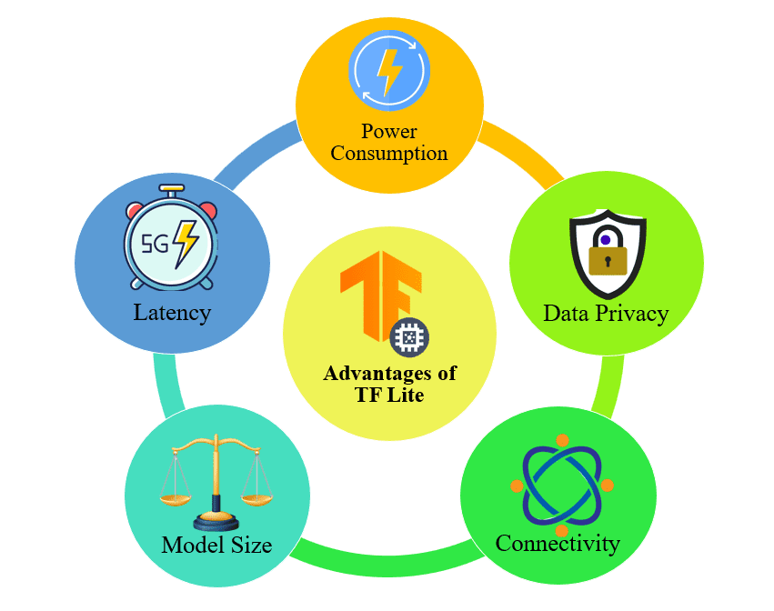
Advantages of using a TensorFlow Lite Model for on-device Machine-Learning:
- Latency: As inference is taken on the edge, there’s no round-trip to a server resulting in low latency.
- Data Privacy: The data is not shared across any net network due to inference at the edge. So the personal information doesn’t leave the device, resolving any concerns about data privacy.
- Connectivity: As no internet connectivity is required, there are no connectivity issues.
- Model Size: TensorFlow Lite models are lightweight as the edge devices are resource-constrained.
- Power Consumptions: Efficient inference and lack of network connectivity lead to low power consumption.
3. Converting TensorFlow Model to TensorFlow Lite Model
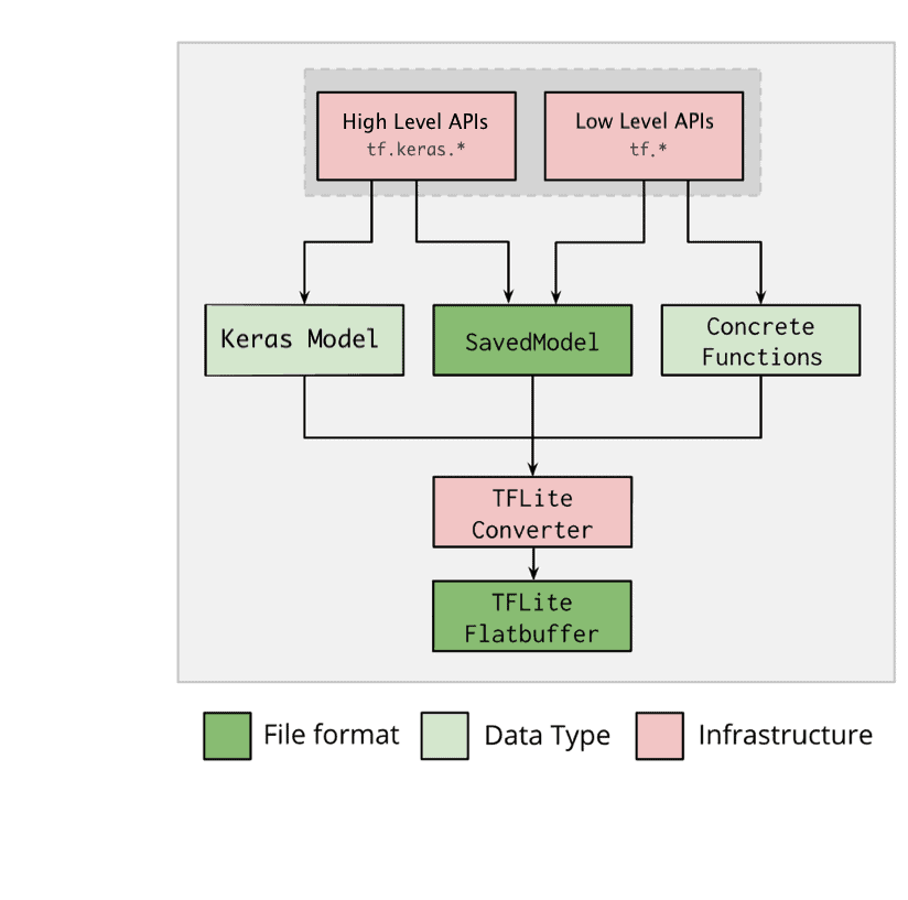
TF Lite Converter converts a TensorFlow model to a TF Lite model. A TF Lite model is represented in a special efficient portable format known as FlatBuffers having a .tflite file extension. This provides several advantages over TensorFlow’s protocol buffer model format, such as reduced size and faster inference. It enables TF Lite to execute efficiently on devices with limited computing and memory resources.
There are several ways to optimize a model. TF Lite currently only solely supports the Quantization technique without needing an external library/dependency. The types of Quantization currently supported by TFLite are :
- Float-16 Quantization
- Integer Quantization
- Dynamic Range Quantization
Before diving deep into these techniques and obtaining the converted TF Lite models, let’s train a base model first. Download the code using the link below. You can also find the entire code in this colab notebook.
4. Base Model Training
Let us train a simple image classifier to classify an image as a cat or dog. This would act as a base model. We will optimize this model and compare the results with the different techniques used. Let’s start by importing the necessary libraries and packages.
# Importing necessary libraries and packages.
import os
import numpy as np
import tensorflow as tf
from tensorflow import keras
import tensorflow_datasets as tfds
from tensorflow.keras.models import Model
import tensorflow_model_optimization as tfmot
from tensorflow.keras.layers import Dropout, Dense, BatchNormalization
%load_ext tensorboard
4.1 Preparing the Dataset
We can directly import the dataset from the TensorFlow Dataset (tfds). Here we will split the dataset into training, validation, and testing set with a split ratio of 0.7:0.2:0.1. The as_supervised parameter is kept True as we need the labels of the images for classification.
# Loading the CatvsDog dataset.
(train_ds, val_ds, test_ds), info = tfds.load('cats_vs_dogs', split=['train[:70%]', 'train[70%:90%]', 'train[90%:]'], shuffle_files=True, as_supervised=True, with_info=True)
Let us now have a look at the dataset information provided in tfds.info(). The dataset has two classes labelled as ‘cat’ and ‘dog’ with 16283, 4653, 2326 training, validation and testing images.
# Obtaining dataset information.
print("Number of  Classes: " + str(info.features['label'].num_classes))
print("Classes : " + str(info.features['label'].names))
NUM_TRAIN_IMAGES = tf.data.experimental.cardinality(train_ds).numpy()
print("Training Images: " + str(NUM_TRAIN_IMAGES))
NUM_VAL_IMAGES = tf.data.experimental.cardinality(val_ds).numpy()
print("Validation Images: " + str(NUM_VAL_IMAGES))
NUM_TEST_IMAGES = tf.data.experimental.cardinality(test_ds).numpy()
print("Testing Images: " + str(NUM_TEST_IMAGES))
Output:
Number of  Classes: 2
Classes : ['cat', 'dog']
Training Images: 16283
Validation Images: 4653
Testing Images: 2326
The function tfds.visualization.show_examples() function displays images and their corresponding labels. It comes very handy when we want to visualize a few images in a single line of code!
# Visualizing the training dataset.
vis = tfds.visualization.show_examples(train_ds, info)
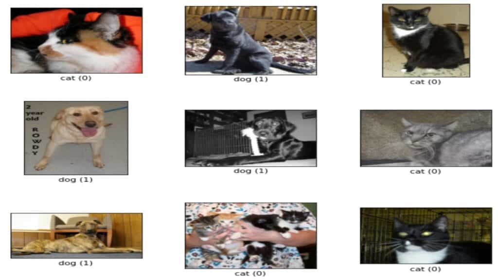
We have chosen 16 as batch size and 224×224 as image size so that the dataset can be processed effectively and efficiently. To prepare the dataset, the images have been resized accordingly.
# Defining batch-size and input image size.
batch_size = 16
img_size = [224, 224]# Resizing images in the dataset.
train_ds = train_ds.map(lambda x, y: (tf.image.resize(x, img_size), y))
val_ds = val_ds.map(lambda x, y: (tf.image.resize(x, img_size), y))
Let’s make sure to use buffered prefetching to yield data from the disk. Prefetching overlaps the preprocessing and model execution of a training step. Doing so reduces the step time to the training and the time it takes to extract the data.
train_ds = train_ds.cache().batch(batch_size).prefetch(buffer_size=10)
val_ds = val_ds.cache().batch(batch_size).prefetch(buffer_size=10)
test_ds = test_ds.cache().batch(batch_size).prefetch(buffer_size=10)
To feed images to the TF Lite model, we need to extract the test images and their labels. We will store them into variables and feed them to TF Lite for evaluation.
# Extracting and saving test images and labels from the test dataset.
test_images = []
test_labels = []
for image, label in test_ds.take(len(test_ds)).unbatch():
  test_images.append(image)
  test_labels.append(label)
4.2 Loading the Model
We have chosen the EfiicientNet B0 model pre-trained on the imagenet dataset for image classification purposes. EfficientNet is a state-of-the-art image classification model. It significantly outperforms other ConvNets.
Let us import the model form tf.keras.applications(). The last layer has been removed by setting include_top = False .We have set the input image size to 224×224 pixels and kept the pooling layer to be GlobalMaxPooling2D. Let’s load the model and unfreeze all the layers to make them trainable.
# Defining the model architecture.
efnet = tf.keras.applications.EfficientNetB0(include_top = False, weights ='imagenet', input_shape = (224, 224, 3), pooling = 'max')# Unfreezing all the layers of the model.
for layer in efnet.layers:
  set_trainable = True
Now, we will add a Dense layer to the pre-trained model and train it. This layer will become the last layer, or the inference layer. We will also add Dropout and BatchNormalization to reduce overfitting.
# Adding Dense, BatchNormalization and Dropout layers to the base model.
x = Dense(512, activation='relu')(efnet.output)
x = BatchNormalization()(x)
x = Dense(64, activation='relu')(x)
x = Dropout(0.2)(x)
predictions = Dense(2, activation='softmax')(x)
4.3 Compiling the Model
We are ready to compile the model. We have used Adam Optimizer with an initial learning rate of 0.0001, sparse categorical cross-entropy as the loss function, and accuracy as the metric. Once compiled, we check the model summary.
# Defining the input and output layers of the model.
model = Model(inputs=efnet.input, outputs=predictions)

# Compiling the model.
model.compile(optimizer=tf.keras.optimizers.Adam(0.0001), loss =tf.keras.losses.SparseCategoricalCrossentropy(from_logits=False), metrics = ["accuracy"])

# Obtaining the model summary.
model.summary()
Output:
=====================================================================Total params: 4,740,453
Trainable params: 4,697,406
Non-trainable params: 43,047
We are using Model Saving Callback and the Reduce LR Callback.
- Model Saving Callback saves the model with the best validation accuracy
- Reduce LR Callback reduces the learning rate by a factor of 0.1 if validation loss remains the same for three consecutive epochs.
# Defining file path of the saved model.
filepath = '/content/model.h5'

# Defining Model Save Callback and Reduce Learning Rate Callback.
model_save = tf.keras.callbacks.ModelCheckpoint(
    filepath,
    monitor="val_accuracy",
    verbose=0,
    save_best_only=True,
    save_weights_only=False,
    mode="max",
    save_freq="epoch")

reduce_lr = tf.keras.callbacks.ReduceLROnPlateau(monitor='loss', factor=0.1, patience=3, verbose=1, min_delta=5*1e-3,min_lr =5*1e-9,)

callback = [model_save, reduce_lr]
4.4 Training the Model
The method model.fit() is called to train the model. We pass the training and validation datasets and train the model for 15 epochs.
# Training the model for 15 epochs.
model.fit(train_ds, epochs=15, steps_per_epoch=(len(train_ds)//batch_size), validation_data=val_ds, validation_steps=(len(val_ds)//batch_size), shuffle=False, callbacks=callback)
4.5 Evaluating the Model
Done training! Let’s check the model’s performance on the test set.
# Evaluating the model on the test dataset.
_, baseline_model_accuracy = model.evaluate(test_ds, verbose=0)
print('Baseline test accuracy:', baseline_model_accuracy*100)
Output:
Baseline test accuracy: 98.53 %
5. Post Training Quantization using TFLite Model
Quantization reduces the precision of the numbers used to represent a model’s parameters, which by default are 32-bit floating-point numbers. This results in smaller model size and faster computation. The following types of quantization are available in TensorFlow Lite:

Let’s explore different types of quantization one by one and compare their performance.
5.1 Float-16 Quantization
In Float-16 quantization, weights are converted to 16-bit floating-point values. This results in a 2x reduction in model size. There is a significant reduction in model size in exchange for minimal impacts to latency and accuracy.
# Passing the Keras model to the TF Lite Converter.
converter = tf.lite.TFLiteConverter.from_keras_model(model)

# Using float-16 quantization.
converter.optimizations = [tf.lite.Optimize.DEFAULT]
converter.target_spec.supported_types = [tf.float16]

# Converting the model.
tflite_fp16_model = converter.convert()

# Saving the model.
with open('/content/fp_16_model.tflite', 'wb') as f:
  f.write(tflite_fp16_model)
We have passed the Float 16 quantization the converter.target_spec.supported_type to specify the type of quantization. The rest of the code remains the same for a general way of conversion for the TF Lite Model. In order to get model accuracy, let’s first define evaluate() function that takes in tflite model and returns model accuracy.
#Function for evaluating TF Lite Model over Test Images
def evaluate(interpreter):
  prediction= []
  input_index = interpreter.get_input_details()[0]["index"]
  output_index = interpreter.get_output_details()[0]["index"]
  input_format = interpreter.get_output_details()[0]['dtype']

  for i, test_image in enumerate(test_images):
    if i % 100 == 0:
      print('Evaluated on {n} results so far.'.format(n=i))
    test_image = np.expand_dims(test_image, axis=0).astype(input_format)
    interpreter.set_tensor(input_index, test_image)

    # Run inference.
    interpreter.invoke()
    output = interpreter.tensor(output_index)
    predicted_label = np.argmax(output()[0])
    prediction.append(predicted_label)

  print('\n')
  # Comparing prediction results with ground truth labels to calculate accuracy.
  prediction = np.array(prediction)
  accuracy = (prediction == test_labels).mean()
  return accuracy
Check this FP-16 Quantized TF Lite’s model performance on the Test Set.
# Passing the FP-16 TF Lite model to the interpreter.
interpreter = tf.lite.Interpreter('/content/fp_16_model.tflite')
# Allocating tensors.
interpreter.allocate_tensors()
# Evaluating the model on the test dataset.
test_accuracy = evaluate(interpreter)
print('Float 16 Quantized TFLite Model Test Accuracy:', test_accuracy*100)
print('Baseline Keras Model Test Accuracy:', baseline_model_accuracy*100)
Output:
Float 16 Quantized TFLite Model Test Accuracy: 98.58 %
Baseline Keras Model Test Accuracy: 98.53 %
5.2 Dynamic Range Quantization
In Dynamic Range Quantization, weights are converted to 8-bit precision values. Dynamic range quantization achieves a 4x reduction in the model size. There is a significant reduction in model size in exchange for minimal impacts to latency and accuracy.
# Passing the baseline Keras model to the TF Lite Converter.
converter = tf.lite.TFLiteConverter.from_keras_model(model)
# Using  the Dynamic Range Quantization.
converter.optimizations = [tf.lite.Optimize.DEFAULT]
# Converting the model
tflite_quant_model = converter.convert()
# Saving the model.
with open('/content/dynamic_quant_model.tflite', 'wb') as f:
  f.write(tflite_quant_model)
Let’s evaluate this TF Lite model on the test dataset.
# Passing the Dynamic Range Quantized TF Lite model to the Interpreter.
interpreter = tf.lite.Interpreter('/content/dynamic_quant_model.tflite')
# Allocating tensors.
interpreter.allocate_tensors()
# Evaluating the model on the test images.
test_accuracy = evaluate(interpreter)
print('Dynamically  Quantized TFLite Model Test Accuracy:', test_accuracy*100)print('Baseline Keras Model Test Accuracy:', baseline_model_accuracy*100)
Output:
Dynamically  Quantized TFLite Model Test Accuracy: 98.15 %
Baseline Keras Model Test Accuracy: 98.53 %
5.3 Integer Quantization
Integer quantization is an optimization strategy that converts 32-bit floating-point numbers (such as weights and activation outputs) to the nearest 8-bit fixed-point numbers. This resulted in a smaller model and increased inferencing speed, which is valuable for low-power devices such as microcontrollers.
The integer quantization requires a representative dataset, i.e. a few images from the training dataset, for the conversion to happen.
# Passing the baseline Keras model to the TF Lite Converter.
converter = tf.lite.TFLiteConverter.from_keras_model(model)
# Defining the representative dataset from training images.
def representative_data_gen():
  for input_value in tf.data.Dataset.from_tensor_slices(test_images).take(100):
    yield [input_value]

converter.optimizations = [tf.lite.Optimize.DEFAULT]
converter.representative_dataset = representative_data_gen

# Using Integer Quantization.
converter.target_spec.supported_ops = [tf.lite.OpsSet.TFLITE_BUILTINS_INT8]

# Setting the input and output tensors to uint8.
converter.inference_input_type = tf.uint8
converter.inference_output_type = tf.uint8
# Converting the model.
int_quant_model = converter.convert()

# Saving the Integer Quantized TF Lite model.
with open('/content/int_quant_model.tflite', 'wb') as f:
  f.write(int_quant_model)
Let’s evaluate the obtained Integer Quantized TF Lite model on the test dataset.
# Passing the Integer Quantized TF Lite model to the Interpreter.
interpreter = tf.lite.Interpreter('/content/int_quant_model.tflite')
# Allocating tensors.
interpreter.allocate_tensors()
# Evaluating the model on the test images.
test_accuracy = evaluate(interpreter)
print('Integer Quantized TFLite Model Test Accuracy:', test_accuracy*100)
print('Baseline Keras Model Test Accuracy:', baseline_model_accuracy*100)
Output:
Integer Quantized TFLite Model Test Accuracy: 92.82 %
Baseline Keras Model Test Accuracy: 98.53 %
6. Performance Evaluation of TFLite Model on Raspberry Pi
The performance of all the converted TF Lite models was evaluated on Raspberry Pi 4, having 4 GB of RAM. The following are the results of the performance evaluation.
6.1 Test Accuracy
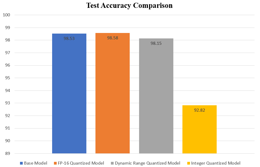
There is a very slight increase in the accuracy of the FP-16 quantized model and a slight decrease in accuracy for the dynamic range quantized model. A very significant amount of dip in the accuracy (~6%) can be observed in the case of the integer quantized model.
6.2 Model Size
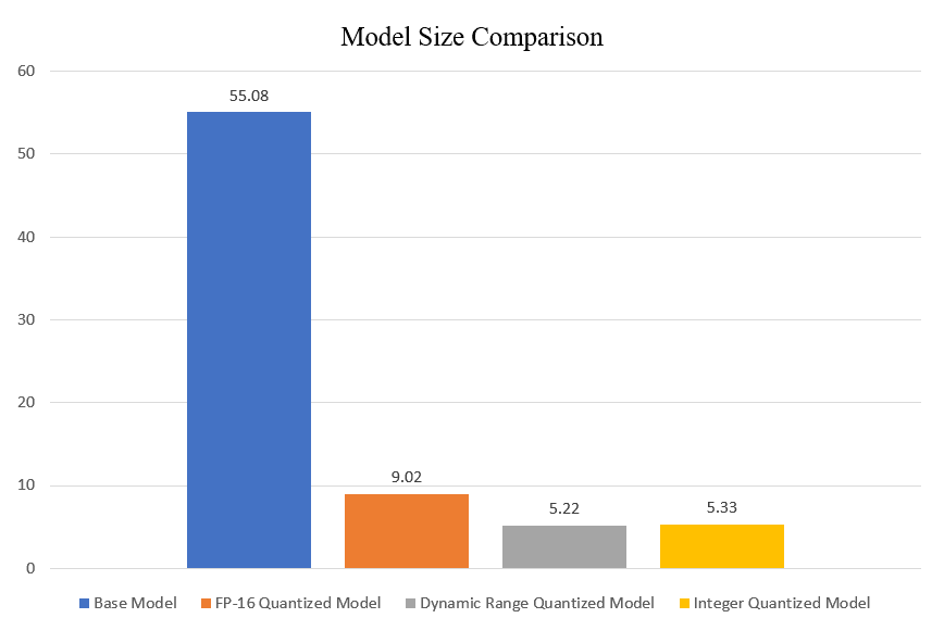
An astonishing 10x reduction in model size was observed in dynamic range and integer quantized models. A 6x reduction in model size was observed in the case of the FP-16 quantized model.
6.3 Inference Time
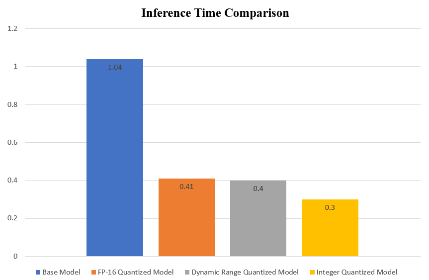
A set of 100 images was randomly chosen from the test dataset to check the inference time of the TF Lite models. The inference time mentioned is the average time taken by a model for inference over 100 images.
The FP-16 quantized model and dynamic range quantized model gave ~2.5x faster inference than the base model. Whereas the integer quantized model gave 3.5x faster inference.




100K+ Learners
Join Free OpenCV Bootcamp3 Hours of Learning