SVM using Scikit-Learn in Python

This post explains the implementation of Support Vector Machines (SVMs) using Scikit-Learn library in Python. We had discussed the math-less details of SVMs in the earlier post.

In this post, we will show the working of SVMs for three different type of datasets:

1. Linearly Separable data with no noise
2. Linearly Separable data with added noise
3. Non-linear separable data with added noise

Prerequisites

Before we begin, we need to install sklearn and matplotlib modules. This can be done using pip.

pip install -U scikit-learn
pip install -U matplotlib

We first import matplotlib.pyplot for plotting graphs. We also need svm imported from sklearn. Finally, from sklearn.model_selection we need train_test_split to randomly split data into training and test sets, and GridSearchCV for searching the best parameter for our classifier. The code below shows the imports.

 
import sys, os
import matplotlib.pyplot as plt
from sklearn import svm
from sklearn.model_selection import train_test_split, GridSearchCV

Linearly separable data with no noise

Let’s first look at the simplest cases where the data is cleanly separable linearly. In the 2D case, it simply means we can find a line that separates the data. In the 3D case, it will be a plane. For higher dimensions, it is simply a plane.

Let’s see how we can use a simple binary SVM classifier based on the data above.

If you have downloaded the code, here are the steps for building a binary classifier

1. Prepare data: We read the data from the files points_class_0.txt and points_class_1.txt. These files simply have x and y coordinates of points — one per line. The points in points_class_0.txt are assinged the label 0 and the points in points_class_1.txt are assigned the label 1. The dataset is then split into training (80%) and test (20%) sets. This dataset is shown in Figure 1.

    
   # Read data
   x, labels = read_data("points_class_0.txt", "points_class_1.txt")
   
   # Split data to train and test on 80-20 ratio
   X_train, X_test, y_train, y_test = train_test_split(x, labels, test_size = 0.2, random_state=0)
   
   # Plot traning and test data
   plot_data(X_train, y_train, X_test, y_test)
   

2. Create an instance of a Linear SVM classifier: Next we create an instance of the Linear SVM classifier from scikit-learn. We use the default parameters because the problem is easy to solve and we expect the default parameters to work just fine. We only specify the SVM be linear.

   # Create a linear SVM classifier 
   clf = svm.SVC(kernel='linear')
   

3. Train a Linear SVM classifier: Next we train a Linear SVM. In other words, based on the training data, we find the line that separates the two classes. This is simply done using the fit method of the SVM class.

   # Train classifier 
   clf.fit(X_train, y_train)
   
   # Plot decision function on training and test data
   plot_decision_function(X_train, y_train, X_test, y_test, clf)
   

   Next, we plot the decision boundary and support vectors. The decision boundary is estimated based on only the traning data. Given a new data point (say from the test set), we simply need to check which side of the line the point lies to classify it as 0 ( red ) or 1 (blue).

   

4. Test a Linear SVM classifier:
   To predict the class of a new point ( or points ) we can simply use the predict method of the SVM class. To obtain the accuracy on the test set, we can use the score method.

   # Make predictions on unseen test data
   clf_predictions = clf.predict(X_test)
   print("Accuracy: {}%".format(clf.score(X_test, y_test) * 100 ))
   

   In this easy example, the accuracy is 100%.

Linearly separable data with noise

Let’s look at a slightly more complicated case shown in Figure 3 where it is not possible to linearly separate the data, but a linear classifier still makes sense. Note that no matter what you do some red points and some blue points will be on the wrong side of the line.

The question now is which line to choose? SVM provides you with parameter called C that you can set while training. In scikit-learn, this can be done using the following lines of code

 
# Create a linear SVM classifier with C = 1
clf = svm.SVC(kernel='linear', C=1)

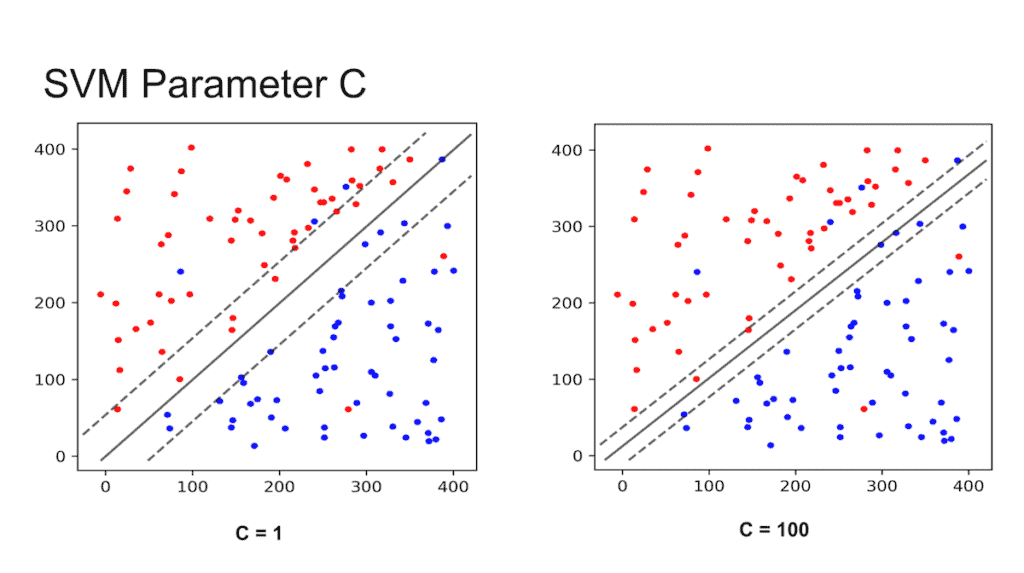
If you set C to be a low value (say 1), the SVM classifier will choose a large margin decision boundary at the expense of larger number of misclassifications. When C is set to a high value (say 100), the classifier will choose a low margin decision boundary and try to minimize the misclassifications. This is shown in Figure 4. The margin is the shown using dotted lines — the larger the space between the dotted lines, the larger is the margin.

You may be tempted to ask which value of C is better. The answer depends on how much noise you think there is in your data. If you think the data is very noisy, you want C to be small. On the other hand, if you think the data is less noisy, you should choose C to be large.

Non-Linearly separable data with noise

Finally, let’s look at data that is impossible to partition using a line.

Is SVM useless in such cases? Fortunately, the answer is no. We can use the Kernel Trick explained in our previous article. In scikit-learn we can specify the kernel type while instantiating the SVM class.

# Create SVM classifier based on RBF kernel. 
clf = svm.SVC(kernel='rbf', C = 10.0, gamma=0.1)

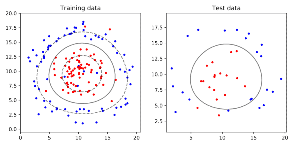
In the above example, we are using the Radial Basis Fucttion expalined in our previous post with parameter gamma set to 0.1. As you can see in Figure 6, the SVM with an RBF kernel produces a ring shaped decision boundary instead of a line.

Looking at Figure 6 you may be tempted to think that using some other value for C and gamma, we may be able to come up with a better decision boundary. Your intuition is right. To find the best parameters, we need to do a parameter sweep by changing values of C and gamma and picking the one that works best. Let’s see how parameters tuning in done using GridSearchCV.

Parameter Tuning using GridSearchCV

The module sklearn.model_selection allows us to do a grid search over parameters using GridSearchCV. All we need to do is specify which parameters we want to vary and by what value. In the following example, the parameters C and gamma are varied. Every combination of C and gamma is tried and the best one is chosen based. The best estimator can be accessed using clf.best_estimator_.

 
# Grid Search
# Parameter Grid
param_grid = {'C': [0.1, 1, 10, 100], 'gamma': [1, 0.1, 0.01, 0.001, 0.00001, 10]}

# Make grid search classifier
clf_grid = GridSearchCV(svm.SVC(), param_grid, verbose=1)

# Train the classifier
clf_grid.fit(X_train, y_train)

# clf = grid.best_estimator_()
print("Best Parameters:\n", clf_grid.best_params_)
print("Best Estimators:\n", clf_grid.best_estimator_)

By default, GridSearchCV performs 3-fold cross-validation. In other words, it divides the data into 3 parts and uses two parts for training, and one part for determining accuracy. This is done three times so each of the three parts is in the training set twice and validation set once. The accuracy for a given C and gamma is the average accuracy during 3-fold cross-validation.

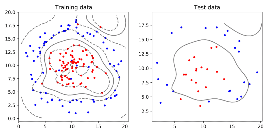
The best parameters ( C = 1 and gamma = 0.01 ) of classifier shown in Figure 7 were found using GridSearchCV. Our intuition also confirms this shape of the decision boundary looks better than the one manually chosen.

Subscribe & Download Code

If you liked this article and would like to download code (C++ and Python) and example images used in this post, please subscribe to our newsletter. You will also receive a free Computer Vision Resource Guide. In our newsletter, we share OpenCV tutorials and examples written in C++/Python, and Computer Vision and Machine Learning algorithms and news.

Subscribe Now