Introduction
Super-resolution refers to the process of upscaling or improving the details of the image. Follow this blog to learn the options for Super Resolution in OpenCV. When increasing the dimensions of an image, the extra pixels need to be interpolated somehow. Basic image processing techniques do not give good results as they do not take the surroundings in context while scaling up. Deep learning and, more recently, GANs come to the rescue here and provide much better results.
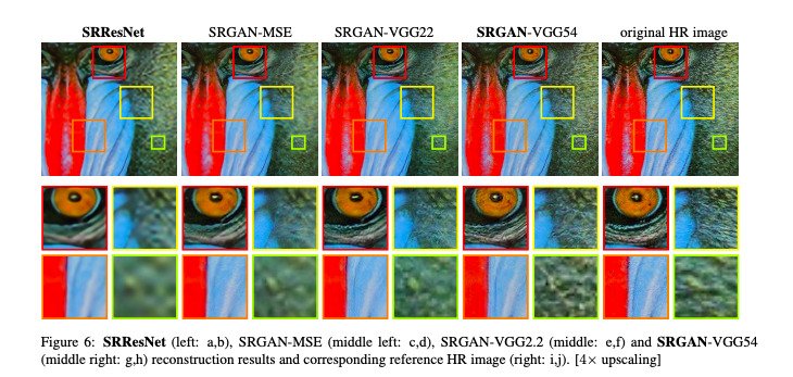
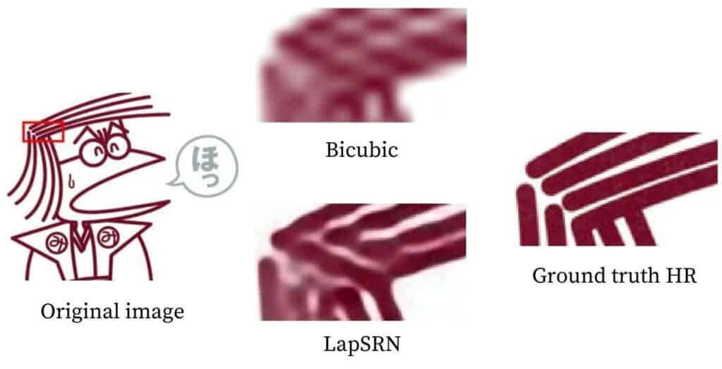
The image given below illustrates super-resolution. The original high-resolution image shows the best details when zoomed in. The other images are achieved after reconstruction after using various super-resolution methods. You can read about them in more detail here.
Super Resolution in OpenCV
OpenCV currently offers a choice of four deep learning algorithms for upscaling images. In this article, all of them will be reviewed. We will also see their results, and compare them with images upscaled using the standard resize operation done in OpenCV using the bicubic interpolation method. The four methods we will discuss are:
Note that the first three algorithms offer an upscale ratio of 2, 3, and 4 times while the last one has 2, 4, and 8 times the original size! The TensorFlow models for each required ratio can be downloaded using the links provided above.
In order to use the above listed models for super resolution, we need to use functionalities additional to the standard OpenCV module. This is why we will have to install opencv-contrib module as well. Further, super resolution is present inside the module dnn_superres (Deep Neural Network based Super Resolution) which was implemented in OpenCV version 4.1 for C++ and OpenCV version 4.3 for Python.
If you already have OpenCV installed, you can check its version using the following code snippet:
import cv2
print(cv2.__version__)
You can also refer to this blog for further details.
If you have an OpenCV version older than 4.3, you can upgrade it using the following command:
pip install opencv-contrib-python --upgradeIn case you do not have OpenCV installed, you can directly install the latest version using pip via the command:
pip install opencv-contrib-pythonNote for advanced users: If you have OpenCV installed already, prefer creating a virtual environment and install opencv-contrib inside that to avoid any dependency issues. This will, by default, install the latest version of OpenCV along with the opencv-contrib module. You can also choose to uninstall OpenCV if you had it previously installed before running this command.
In order to compare the above mentioned algorithms we will be using the below image as reference – specifically we will try to generate a high resolution image of the OpenCV logo present in the top right corner of the image to give you an idea of super-resolution capabilities of the OpenCV super-res module.
Code
Python
import cv2
import matplotlib.pyplot as plt
# Read image
img = cv2.imread("AI-Courses-By-OpenCV-Github.png")
plt.imshow(img[:,:,::-1])
plt.show()
We first import opencv and matplotlib and read the test-image. To crop out the OpenCV logo, we use the code given below.
# Cropout OpenCV logo
img = img[:80,850:]
plt.imshow(img[:,:,::-1])
plt.show()
C++
// Read image
Mat img = imread("AI-Courses-By-OpenCV-Github.png");
// Region to crop
Rect roi;
roi.x = 850;
roi.y = 0;
roi.width = img.size().width - 850;
roi.height = 80;
img = img(roi);
EDSR
Lim et al. proposed two methods in their paper, EDSR, and MDSR. Different models are required for different scales in the EDSR method. In comparison a single model can reconstruct various scales in the MDSR model. However, in this article, we will discuss only EDSR.
A ResNet style architecture is used without the Batch Normalization layers. They found that those layers get rid of range flexibility from the features’ networks, improving the performance. This allows them to build a larger model with better performance. To counter the instability found in large models, they used residual scaling with a factor of 0.1 in each residual block by placing constant scaling layers after the last convolutional layers. Also, ReLu activation layers are not used after the residual blocks.
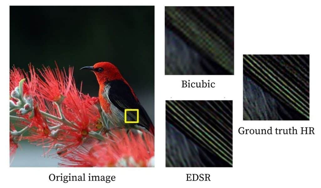
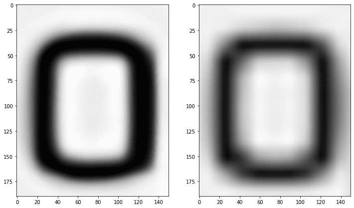
The architecture is initially employed for a scaling factor of 2. Then these pre-trained weights are used when training for a scaling factor of 3 and 4. This not only accelerates the training but also improves the performance of the models. The image below is a comparison of the 4x super-resolution result of the EDSR method, bicubic interpolation method and the original high-resolution image.
Code
Python
sr = cv2.dnn_superres.DnnSuperResImpl_create()

path = "EDSR_x4.pb"

sr.readModel(path)

sr.setModel("edsr",4)

result = sr.upsample(img)

# Resized image
resized = cv2.resize(img,dsize=None,fx=4,fy=4)

plt.figure(figsize=(12,8))
plt.subplot(1,3,1)
# Original image
plt.imshow(img[:,:,::-1])
plt.subplot(1,3,2)
# SR upscaled
plt.imshow(result[:,:,::-1])
plt.subplot(1,3,3)
# OpenCV upscaled
plt.imshow(resized[:,:,::-1])
plt.show()
C++
#include <iostream>
#include <opencv2/dnn_superres.hpp>
#include <opencv2/imgproc.hpp>
#include <opencv2/highgui.hpp>

using namespace std;
using namespace cv;
using namespace dnn;
using namespace dnn_superres;

Mat upscaleImage(Mat img, string modelName, string modelPath, int scale){
	DnnSuperResImpl sr;
	sr.readModel(modelPath);
	sr.setModel(modelName,scale);
	// Output image
	Mat outputImage;
	sr.upsample(img, outputImage);
	return outputImage;
}

int main(int argc, char *argv[])
{
	// Read image
	Mat img = imread("AI-Courses-By-OpenCV-Github.png");
	// Region to crop
	Rect roi;
	roi.x = 850;
	roi.y = 0;
	roi.width = img.size().width - 850;
	roi.height = 80;
	img = img(roi);

	// EDSR (x4)
	string path = "EDSR_x4.pb";
	string modelName = "edsr";
	int scale = 4;
	Mat result = upscaleImage(img, modelName, path, scale);

	// Image resized using OpenCV
	Mat resized;
	cv::resize(img, resized, cv::Size(), scale, scale);

	imshow("Original image",img);
	imshow("SR upscaled",result);
	imshow("OpenCV upscaled",resized);
	waitKey(0);
	destroyAllWindows();

	return 0;
}

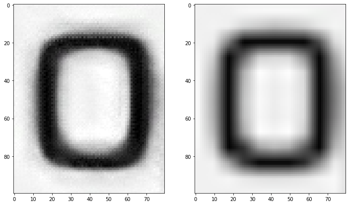
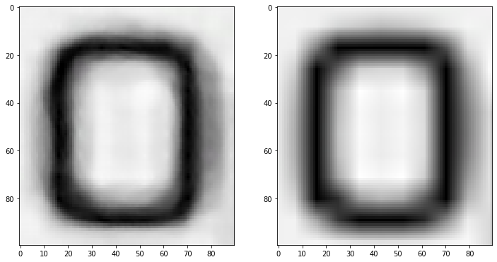
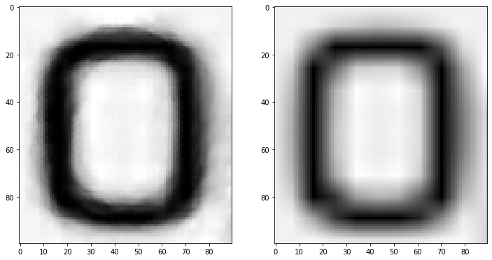
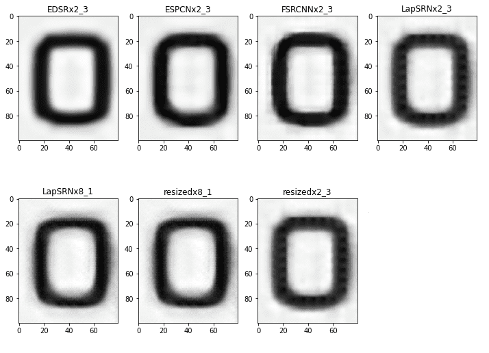
To help you visualize super-resolution capabilities even better, let us take a look at a specific letter and compare the results. Let’s zoom into the letter “O” in OpenCV.
ESPCN
Instead of performing super-resolution after upscaling the low resolution using a bicubic filter, Shi et al. extract feature maps in the low resolution itself and use complex upscaling filters to get the result. The upscaling layers are only deployed at the end of the network. This ensures that the complex operations occurring in the model happen on lower dimensions, which makes it fast, especially compared to other techniques.
The base structure of ESPCN is inspired by SRCNN. Instead of using the customary convolution layers, sub-pixel convolution layers are utilized, which act like deconvolution layers. The sub-pixel convolution layer is utilized in the last layer to produce the high-resolution map. Along with this, they found that the Tanh activation function works much better than the standard ReLu function.
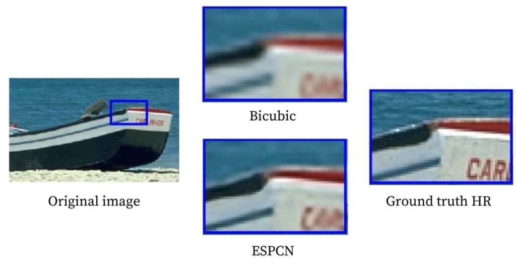
The image below is a comparison of 3x super-resolution result of the ESPCN method, bicubic interpolation method and the original high resolution image.
Code
Python
sr = cv2.dnn_superres.DnnSuperResImpl_create()

path = "ESPCN_x3.pb"

sr.readModel(path)

sr.setModel("espcn",3)

result = sr.upsample(img)

# Resized image
resized = cv2.resize(img,dsize=None,fx=3,fy=3)

plt.figure(figsize=(12,8))
plt.subplot(1,3,1)
# Original image
plt.imshow(img[:,:,::-1])
plt.subplot(1,3,2)
# SR upscaled
plt.imshow(result[:,:,::-1])
plt.subplot(1,3,3)
# OpenCV upscaled
plt.imshow(resized[:,:,::-1])
plt.show()
C++
#include <iostream>
#include <opencv2/dnn_superres.hpp>
#include <opencv2/imgproc.hpp>
#include <opencv2/highgui.hpp>

using namespace std;
using namespace cv;
using namespace dnn;
using namespace dnn_superres;

Mat upscaleImage(Mat img, string modelName, string modelPath, int scale){
	DnnSuperResImpl sr;
	sr.readModel(modelPath);
	sr.setModel(modelName,scale);
	// Output image
	Mat outputImage;
	sr.upsample(img, outputImage);
	return outputImage;
}

int main(int argc, char *argv[])
{
	// Read image
	Mat img = imread("AI-Courses-By-OpenCV-Github.png");
	// Region to crop
	Rect roi;
	roi.x = 850;
	roi.y = 0;
	roi.width = img.size().width - 850;
	roi.height = 80;
	img = img(roi);

	// ESPCN (x3)
	string path = "ESPCN_x3.pb";
	string modelName = "espcn";
	int scale = 3;
	Mat result = upscaleImage(img, modelName, path, scale);

	// Image resized using OpenCV
	Mat resized;
	cv::resize(img, resized, cv::Size(), scale, scale);

	imshow("Original image",img);
	imshow("SR upscaled",result);
	imshow("OpenCV upscaled",resized);
	waitKey(0);
	destroyAllWindows();

	return 0;
}

FSRCNN
FSRCNN and ESPCN have very similar concepts. Both of them have their base structure inspired by SRCNN and employ upscaling layers at the end for speed instead of interpolating it early on. Furthermore, they even shrink the input feature dimension and use smaller filter sizes before finally using more mapping layers, which results in the model being even smaller and faster.
The architecture starts with convolutional layers, with its filter size dropped to 5 from the 9 of SRCNN. Shrinking layers are applied as the input resolution itself can be huge and take much time. Filter size of 1×1 is used, which does not increase the computational cost.
The authors next focus on reducing the non-linear mapping that plays an integral part in slowing down the model without compromising accuracy. Hence, they use multiple 3×3 filters. The next expanding section is the opposite of the shrinking section, before finally applying deconvolutional layers for upsampling. For the activation function, PReLu was used.
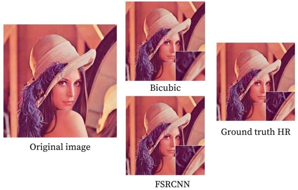
The image below is a comparison of 3x super-resolution result of the FSRCNN method, bicubic interpolation method and the original high resolution image.
Code
Python
sr = cv2.dnn_superres.DnnSuperResImpl_create()

path = "FSRCNN_x3.pb"

sr.readModel(path)

sr.setModel("fsrcnn",3)

result = sr.upsample(img)

# Resized image
resized = cv2.resize(img,dsize=None,fx=3,fy=3)

plt.figure(figsize=(12,8))
plt.subplot(1,3,1)
# Original image
plt.imshow(img[:,:,::-1])
plt.subplot(1,3,2)
# SR upscaled
plt.imshow(result[:,:,::-1])
plt.subplot(1,3,3)
# OpenCV upscaled
plt.imshow(resized[:,:,::-1])
plt.show()
C++
#include <iostream>
#include <opencv2/dnn_superres.hpp>
#include <opencv2/imgproc.hpp>
#include <opencv2/highgui.hpp>

using namespace std;
using namespace cv;
using namespace dnn;
using namespace dnn_superres;

Mat upscaleImage(Mat img, string modelName, string modelPath, int scale){
	DnnSuperResImpl sr;
	sr.readModel(modelPath);
	sr.setModel(modelName,scale);
	// Output image
	Mat outputImage;
	sr.upsample(img, outputImage);
	return outputImage;
}

int main(int argc, char *argv[])
{
	// Read image
	Mat img = imread("AI-Courses-By-OpenCV-Github.png");
	// Region to crop
	Rect roi;
	roi.x = 850;
	roi.y = 0;
	roi.width = img.size().width - 850;
	roi.height = 80;
	img = img(roi);

	// FSRCNN (x3)
	string path = "FSRCNN_x3.pb";
	string modelName = "fsrcnn";
	int scale = 3;
	Mat result = upscaleImage(img, modelName, path, scale);

	// Image resized using OpenCV
	Mat resized;
	cv::resize(img, resized, cv::Size(), scale, scale);

	imshow("Original image",img);
	imshow("SR upscaled",result);
	imshow("OpenCV upscaled",resized);
	waitKey(0);
	destroyAllWindows();

	return 0;
}

LapSRN
LapSRN offers a middle ground between the contrasting strategies of upscaling at the start and end. It proposes to upscale gently till the end. Its name is based on Laplacian pyramids, and the architecture is basically like a pyramid upscaling the lower resolution image until the end. For speed, parameter sharing is heavily relied on; and just like the EDSR models, they also proposed a single model that can reconstruct different scales calling it MS-LapSRN. However, in this article, we will discuss only LapSRN.
The models consist of two branches: feature extraction and an image reconstruction branch. Parameter sharing occurs among the different scales, i.e., 4x uses parameters from 2x model and so on. This means that one pyramid is used for scaling 2x, two for 4x, and three for 8x! Making such deep models means they can suffer from gradient vanishing problems. So they try different types of local skip connections like distinct-source skip connections and shared-source connections. Charbonnier loss is used for the model’s loss function, and batch normalization layers are not used.
The image below is a comparison of 8x super-resolution result of LapSRN method, bicubic interpolation method and the original high resolution image.
Code
Python
sr = cv2.dnn_superres.DnnSuperResImpl_create()

path = "LapSRN_x8.pb"

sr.readModel(path)

sr.setModel("lapsrn",8)

result = sr.upsample(img)

# Resized image
resized = cv2.resize(img,dsize=None,fx=8,fy=8)

plt.figure(figsize=(12,8))
plt.subplot(1,3,1)
# Original image
plt.imshow(img[:,:,::-1])
plt.subplot(1,3,2)
# SR upscaled
plt.imshow(result[:,:,::-1])
plt.subplot(1,3,3)
# OpenCV upscaled
plt.imshow(resized[:,:,::-1])
plt.show()
C++
#include <iostream>
#include <opencv2/dnn_superres.hpp>
#include <opencv2/imgproc.hpp>
#include <opencv2/highgui.hpp>

using namespace std;
using namespace cv;
using namespace dnn;
using namespace dnn_superres;

Mat upscaleImage(Mat img, string modelName, string modelPath, int scale){
	DnnSuperResImpl sr;
	sr.readModel(modelPath);
	sr.setModel(modelName,scale);
	// Output image
	Mat outputImage;
	sr.upsample(img, outputImage);
	return outputImage;
}

int main(int argc, char *argv[])
{
	// Read image
	Mat img = imread("AI-Courses-By-OpenCV-Github.png");
	// Region to crop
	Rect roi;
	roi.x = 850;
	roi.y = 0;
	roi.width = img.size().width - 850;
	roi.height = 80;
	img = img(roi);

	// LapSRN (x2)
	string path = "LapSRN_x8.pb";
	string modelName = "lapsrn";
	int scale = 8;
	Mat result = upscaleImage(img, modelName, path, scale);

	// Image resized using OpenCV
	Mat resized;
	cv::resize(img, resized, cv::Size(), scale, scale);

	imshow("Original image",img);
	imshow("SR upscaled",result);
	imshow("OpenCV upscaled",resized);
	waitKey(0);
	destroyAllWindows();

	return 0;
}

Generic Code
The first step is to create an object of the DNN superresolution class. This is followed by the reading and setting of the model, and finally, the image is upscaled.
We have provided the Python and C++ codes below. You can replace the value of the model_path variable with the path of the model that you want to use. We have already provided the links to all models at the beginning of the blog. They are also provided below for ready reference.
C++
#include <opencv2/dnn_superres.hpp>

DnnSuperResImpl sr;
string model_path = "ESPCN_x4.pb";
sr.readModel(model_path);
sr.setModel("espcn", 4); // set the model by passing the value and the upsampling ratio
Mat result; // creating blank mat for result
sr.upsample(img, result); // upscale the input image
Python
import cv2

sr = cv2.dnn_superres.DnnSuperResImpl_create()
path = "ESPCN_x4.pb"
sr.readModel(path)
sr.setModel("espcn", 4) # set the model by passing the value and the upsampling ratio
result = sr.upsample(img) # upscale the input image
Note: Make to sure to pass the model name correctly in the lower case along with the correct upsampling ratio as the model taken in sr.setModel().
Results

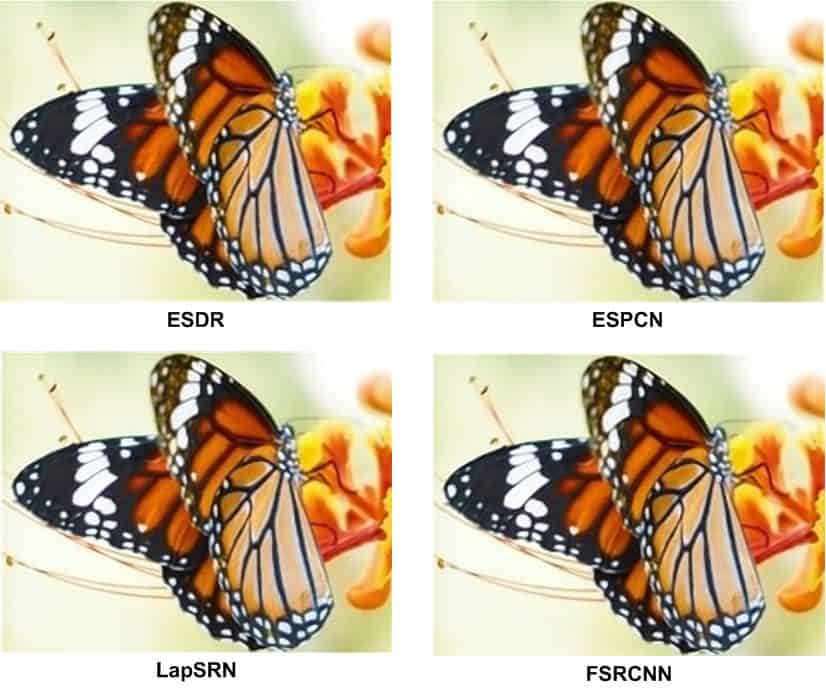
To show the results here, only the butterfly region from the above image is cropped out. It is upscaled four times using the super-resolution models and presented in the table below.
To get a clearer idea of the results, let’s compare all the results we have obtained from our code. To compare images of equal size, the EDSR, ESPCN, FSRCNN model results have been resized thrice.
It is not easy to differentiate between the results with the naked eye by just upscaling the images. So to validate all the model’s performance, these techniques were applied to three images having a size of 500×333 and were downscaled to the required dimension before upsampling it back to 500×333. The upscaled images were then compared with the original image using PSNR and SSIM. The mean results of all the images were calculated and are given below.
| Name | 2x | 3x | 4x | 8x |
| Bicubic | 27.8667 | 25.9653 | 24.7637 | 21.5657 |
| EDSR | 28.5503 | 26.484 | 25.3513 | – |
| ESPCN | 28.3803 | 25.9613 | 25.0947 | – |
| FSRCNN | 28.1673 | 26.128 | 25.0683 | – |
| LapSRN | 28.098 | – | 25.053 | 21.587 |
| Name | 2x | 3x | 4x | 8x |
| Bicubic | 0.859 | 0.794 | 0.728 | 0.552 |
| EDSR | 0.885 | 0.825 | 0.762 | – |
| ESPCN | 0.877 | 0.799 | 0.736 | – |
| FSRCNN | 0.876 | 0.798 | 0.735 | – |
| LapSRN | 0.874 | – | 0.735 | 0.554 |
Moreover, the time taken on an Intel i5-7200U is also logged, and the mean of all images is given below. Keep in mind that the image size passed to 3x is smaller than 2x and is the same case with even larger scaling factors.
| Name | 2x | 3x | 4x | 8x |
| Bicubic | 0.00099 | 0.00099 | 0.00098 | 0.00098 |
| EDSR | 32.501 | 16.718 | 10.224 | – |
| ESPCN | 0.049 | 0.032 | 0.018 | – |
| FSRCNN | 0.074 | 0.035 | 0.054 | – |
| LapSRN | 0.501 | – | 0.742 | 0.765 |
For a more detailed benchmark, of these methods, refer to this article on OpenCV’s documentation.
Applications
Super-resolution is not just a tool that would bring sci-fi or crime movies detection to reality. The applications of super resolution are spread across various fields.
Medical Imaging: Super-resolution is a great solution to improving the quality of X-Rays, CT Scans, etc. It helps highlight important details about the anatomical and functional information of the human body. Improving the resolution or enhancing medical images also helps in highlighting critical blockages or tumours.
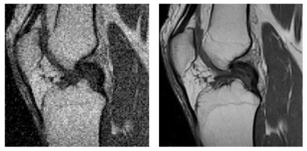
Left original LR image Right SR result image Source
Multimedia, Image, and Video Processing Applications: Super-resolution can convert few hazy frames from a cell-phone video into clearly readable images or snapshots.
Biometric Identification: Super-resolution can play a crucial role in biometric recognition by enhancement for face, fingerprint and iris images. The shape, structure and texture are greatly enhanced which helps in distinctly identifying a biometric print.
Remote Sensing: The concept of using super-resolution in remote sensing and satellite imaging has been developed for decades. In fact, the first super-resolution idea was motivated by the need for better quality and resolution of Landsat remote sensing images.
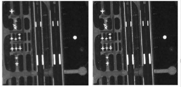
Left original LR image Right SR result image Source
Astronomical imaging: Improving the resolution of astronomical pictures helps in focusing on tiny details that could turn out to be significant discoveries in outer space.
Surveillance Imaging: Traffic surveillance and security systems play a very important role in maintaining civilian safety. Applying super-resolution on digitally recorded videos goes a long way in identifying traffic or security violations.
Conclusion
In this blog, we have given a brief introduction into the concept of Super-Resolution. We chose four Super Resolution models, discussed their architecture and results to highlight the variety of choice for image super-resolution and the efficiency of these methods.
To summarize our observations, EDSR comfortably gives the best results out of the four methods. However, it is slow and cannot be used for real-time applications. ESPCN and FSRCNN are the go-to methods if real-time performance is desired and have almost identical performances. However, ESPCN slightly edges ahead of FSRCNN for the images used. For an upscaling factor of 8x, even though a combination of 2x and 4x models can be used, the 8x upscaling model of LapSRN performs better in most situations. Although none of these methods can match the traditional bicubic method speed, they certainly give better results.







100K+ Learners
Join Free OpenCV Bootcamp3 Hours of Learning