Object detection has come a long way, especially with the rise of transformer-based models. RF-DETR, developed by Roboflow, is one such model that offers both speed and accuracy. Using Roboflow’s tools makes the process even easier. Their platform handles everything from uploading and annotating data to exporting it in the right format. This means less time setting things up and more time training and improving your model.
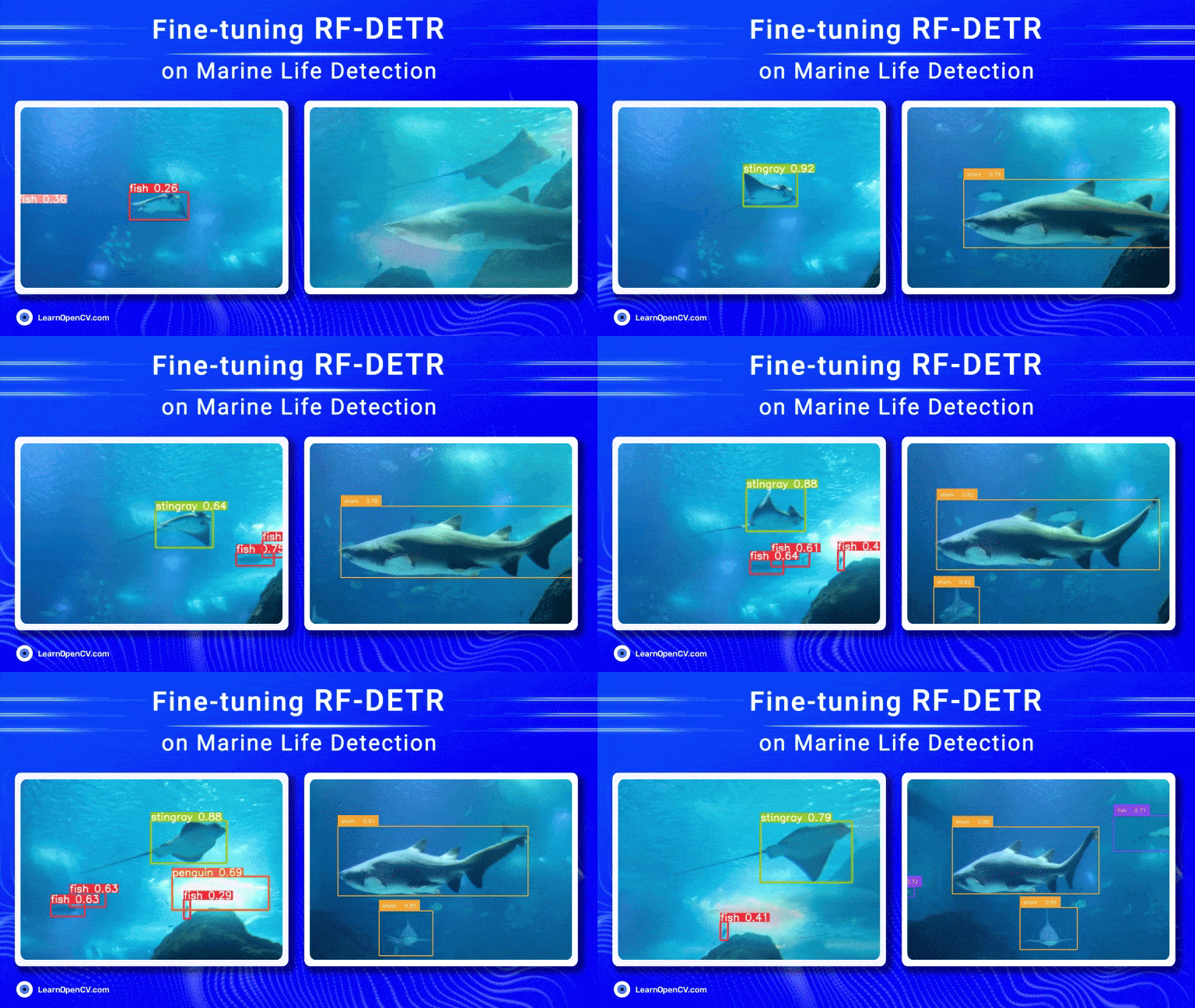
In this blog, we’ll look at how RF-DETR works, its architecture, and fine-tuning it to perform well on an underwater dataset. We will also work with tools like Supervision that can help in improving results through smart data handling and visualization.
- Model variants, performance, and benchmarking
- Architecture Overview
- Inference Results
- Fine-tuning on aquatic dataset
- Key Takeaways
- Conclusion
- References
Model variants, performance, and benchmarking
RF-DETR is a real-time, transformer-based object detection model architecture developed by Roboflow and released under the Apache 2.0 license.
RF-DETR can exceed 60 AP(average Precision) on the Microsoft COCO benchmark alongside competitive performance at base sizes. It also achieves state-of-the-art performance on RF100-VL, an object detection benchmark that measures model domain adaptability to real-world problems. RF-DETR has a speed comparable to current real-time objection models.
RF-DETR is available in two model sizes: RF-DETR-Base (29M parameters) and RF-DETR-large(128M parameters). The base variant is best for fast inferencing, and the large version is best for the most accurate predictions, but it takes longer to compute than the base variant.
RF-DETR is small enough to run on the edge, making it ideal for deployments requiring strong accuracy and real-time performance.
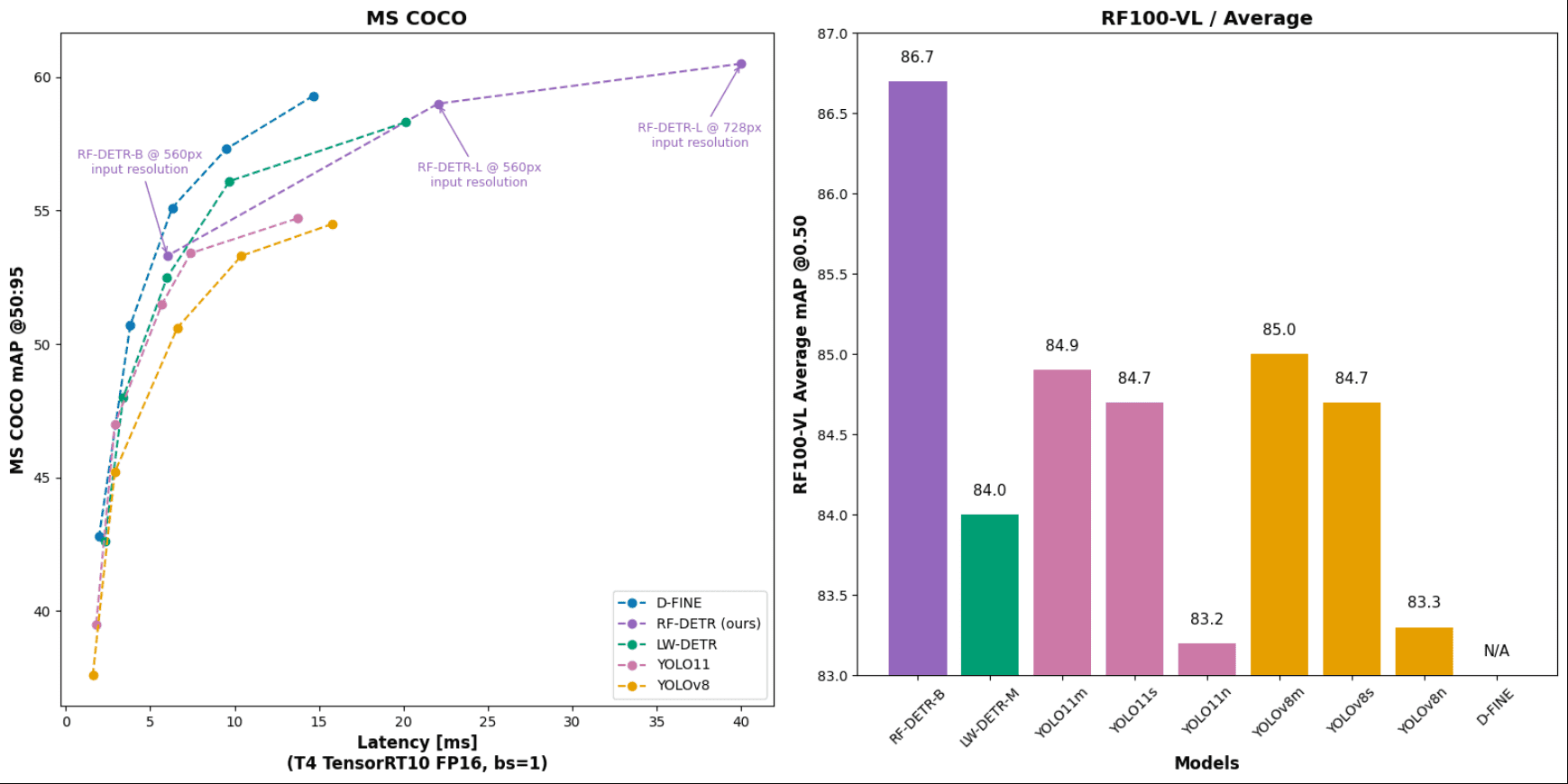
| Model | Params (M) | mAP(coco) @0.50:0.95 | mAP(rf100-vl) average @0.50 | mAP(rf100-vl) average @0.50:0.95 | Total Latency(ms) T4, bs = 1 |
| D-FINE-M | 19.3 | 55.1 | N/A | N/A | 6.3 |
| LW-DETR-M | 28.3 | 52.5 | 84.0 | 57.5 | 6.0 |
| YOLO11m | 20.0 | 51.5 | 84.9 | 59.7 | 5.7 |
| YOLOv8m | 28.9 | 50.6 | 85.0 | 59.8 | 6.3 |
| RF-DETR-B | 29.0 | 53.3 | 86.7 | 60.3 | 6.0 |
Architecture Overview
CNN remains the core component of many of the best real-time object detection approaches, including models like D-FINE that leverage both CNNs and Transformers in their architecture.
Recently, through the introduction of RT-DETR in 2023, the DETR family of models supported by transformer architecture has shown comparable and surpassing results on end-to-end object detection tasks by eliminating hand-designed components like anchor generation and non-maximum suppression (NMS), which were standard in frameworks like Faster-RCNN.
Despite the advantages offered by DETR models, it suffers from two significant limitations:
- Slow Convergence
- Poor Performance on Small Objects
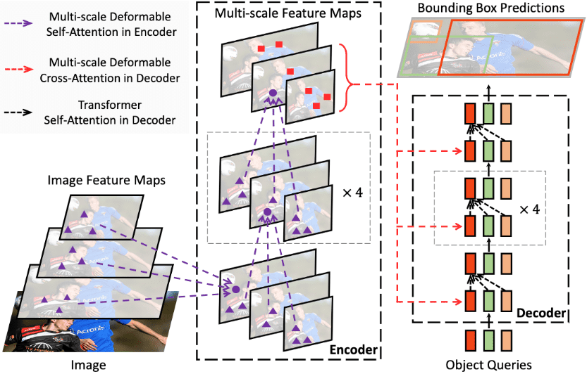
RF-DETR compensates for the above limitations using an architecture based on the Deformable DETR model. However, unlike Deformable DETR, which uses a multi-scale self-attention mechanism, RF-DETR extracts image feature maps from a single-scale backbone.
RF-DETR combines LW-DETR with a pre-trained DINOv2 backbone. Utilizing DINOv2 pre-trained backbone provides exceptional ability to adapt to novel domains based on the knowledge stored in the pre-trained model.
Let’s examine the architectural details of LW-DETR architecture, which is adopted in RF-DETR along with DINOv2. The architectural details of DINOv2 are beyond the scope of this article. For those interested in grasping the ideologies and architecture of DINOv2, visit our article on learnopencv, which covers paper explanation and road segmentation implementation in one.
LW-DETR
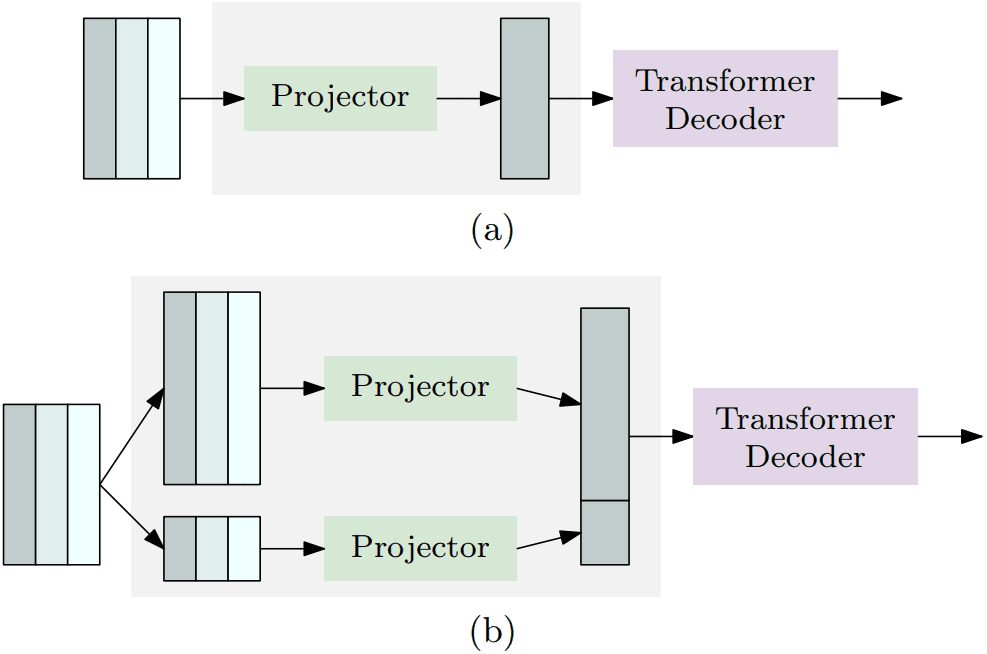
LW-DETR’s architecture consists of a simple stack of a ViT encoder, a projector, and a shallow DETR decoder. It explores the feasibility of plain ViT backbones and a DETR framework for real-time detection.
Encoder:
The paper’s authors used vanilla ViT for the detection encoder. A plain ViT consists of a patchification layer and transformer encoder layers. A transformer encoder layer in the initial ViT contains a global self-attention layer over all the tokens and an FFN layer. Global self-attention is computationally costly, and its time complexity is quadratic to the number of tokens.
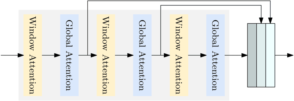
Hence, the authors instead introduced window self-attention to reduce the computational complexity; they also proposed the aggregation of multi-level feature maps, the intermediate and final feature maps in the encoder, forming stronger encoded feature maps.
Decoder:
The decoder is a stack of transformer decoder layers. Each layer consists of self-attention, cross-attention, and FFN. We adopt deformable cross-attention for computational efficiency.DETR and its variants usually adopt six decoder layers. Still, the authors explained that using only three transformer decoder layers can lead to a time reduction from 1.4 ms to 0.7 ms, which is significant compared to the time cost of 1.3 ms of the remaining part for the tiny version in their approach.
They adopted a mixed query selection scheme to form the object queries in addition to content queries and spatial queries. The content queries are learnable embeddings, similar to DETR. The spatial queries are based on a two-stage scheme: selecting top-K features from the last layer in the Projector, predicting the bounding boxes, and transforming the corresponding boxes into embeddings as spatial queries.
Projector:
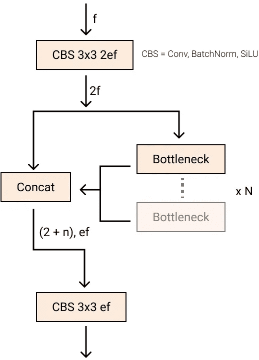
The projector connects the encoder and decoder. It takes the aggregated encoded feature maps from the encoder as input. The projector is a C2f block implemented in YOLOv8.
For large and x-large versions of LW-DETR, the projector is modified to output two-scale feature maps, and the multi-scale decoder is used accordingly. The projector contains two parallel C2f blocks. One processes ⅛ feature maps, which are obtained by upsampling the input through a deconvolution, and the other processes 1/32 maps, which are obtained by downsampling the input through a stride convolution.
Inference Results
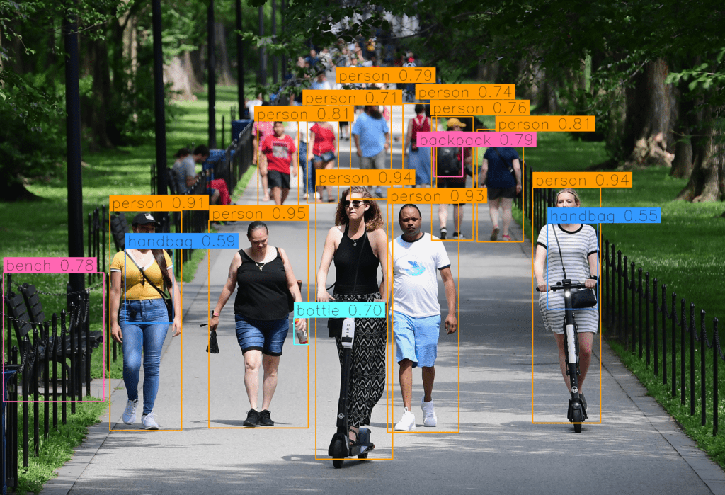
Let’s examine how the model performs out of the box by writing a simple inferencing script provided by Roboflow.
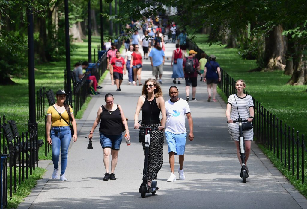
We will use the script below to detect objects in the image provided above.
One thing to note is that we will use the Supervision library created and maintained by Roboflow. This library is easy to use and doesn’t require much overhead to understand the various functionality it provides for object detection tasks. Whether you need to load your dataset from your hard drive, draw detections on an image or video, or count how many detections are in a zone, you can always count on Supervision!!
Let’s begin some coding. 🙂
There are requirements to install before performing inferencing. If you are working on VS code or terminal, it is highly recommended that you create your virtual environment and work inside it for better consistency and fewer dependency issues.
!pip install -q rf-detr==1.1.0
If you are working in colab, integrate the API key of Roboflow in your working environment like the one shown below.
- Go to the Roboflow settings page and click copy.
- In Colab, go to the left panel and click on
secrets(🔑).- Store the Roboflow API key under the name ROBOFLOW_API_KEY.
import os
from google.colab import userdata

os.environ["ROBOFLOW_API_KEY"] = userdata.get("ROBOFLOW_API_KEY")
Now, we are all set to start the inferencing.
#importing necessary libraries
from rfdetr import RFDETRBase
import supervision as sv
from rfdetr.util.coco_classes import COCO_CLASSES
import numpy as np
from PIL import Image

#instantiating model object, the corresponding COCO pretrained checkpoints are automatically loaded when you initialize either class.
model = RFDETRBase()

#reading image using Pillow library, OpenCV or Matplotlib can also be used
image = Image.open("path_to_your_input_image")

#performing inferencing, threshold decides the minimum confidence score each bbox should have
detections = model.predict(image, threshold = 0.5)

#visualizing the result using Supervision library
color = sv.ColorPalette.from_hex([
    "#ffff00", "#ff9b00", "#ff8080", "#ff66b2", "#ff66ff", "#b266ff",
    "#9999ff", "#3399ff", "#66ffff", "#33ff99", "#66ff66", "#99ff00"
])
text_scale = sv.calculate_optimal_text_scale(resolution_wh=image.size)
thickness = sv.calculate_optimal_line_thickness(resolution_wh=image.size)

bbox_annotator = sv.BoxAnnotator(color=color, thickness=thickness)
label_annotator = sv.LabelAnnotator(
    color=color,
    text_color=sv.Color.BLACK,
    text_scale=text_scale,
    smart_position=True
)

labels = [
    f"{COCO_CLASSES[class_id]} {confidence:.2f}"
    for class_id, confidence
    in zip(detections.class_id, detections.confidence)
]

#displaying the result
annotated_image = image.copy()
annotated_image = bbox_annotator.annotate(annotated_image, detections)
annotated_image = label_annotator.annotate(annotated_image, detections, labels)
annotated_image
Fine-tuning on aquatic dataset
While RF-DETR demonstrates strong performance on general benchmarks like COCO and shows promise in domain adaptability, the challenge is applying it to specific, niche domains.
Fine-tuning RF-DETR on aquatic imagery datasets is a powerful way to adapt the model to new environments and object classes. Leveraging Roboflow’s tools and resources, you can streamline the process from dataset preparation to training configurations and visualizing the results.
One important thing to note before we start fine-tuning our aquatic dataset is that Roboflow has designed its fine-tuning pipeline so that datasets in COCO format can only be used for training. COCO format:
underwater_COCO_dataset/
├── train/
│   ├── images/
│   │   ├── image1.jpg
│   │   ├── image2.jpg
│   │   └── ...
│   └── _annotations.coco.json
├── val/
│   ├── images/
│   │   ├── image1.jpg
│   │   ├── image2.jpg
│   │   └── ...
│   └── _annotations.coco.json
└── test/
    ├── images/
    │   ├── image1.jpg
    │   ├── image2.jpg
    │   └── ...
    └── _annotations.coco.json
The Challenge: Underwater Animal Detection
Our chosen dataset comprises images of underwater animals of various species, such as fish, jellyfish, penguin, puffin, shark, starfish and stingray.
This domain poses different challenges as compared to typical terrestrial datasets, namely:
- Varying Visibility
- Camouflage
- Scale Variation: Detecting both small, distant fish and larger, closer fish
This dataset is publicly available to all people on the Kaggle Platform and can be saved locally on your machine or imported into a new Kaggle notebook.
A few essential details about the dataset:
- Already split into the train, validation, and test sets
- Consists of 638 images. Annotations (Ground Truth) are in YOLO format (
class_id,x_centre,y_centre,width,height) - Pre-processing steps applied to each image:
- Auto-orientation of pixel data (with EXIF-orientation stripping)
- Resize to 1024 x 1024 (fit within this range)
Now that we know the dataset must be in COCO format, let’s start writing a script to convert our aquatic dataset from YOLO format to COCO format. We will also provide the script for conversion in this blog, which you can download and work around.
Lets begin…..
import json
import os
from PIL import Image
The first step after importing all the required libraries involves defining a list of dictionaries with the name of the class and corresponding ID as dict_keys.
#including supercategory is optional and can be eleminated.
categories = [{"id": 0, "name": 'fish', "supercategory": "animal"},
{"id": 1, "name": 'jellyfish', "supercategory": "animal"},
{"id": 2, "name": "penguin", "supercategory": "animal"},
{"id": 3, "name": "puffer_fish", "supercategory": "animal"},
{"id": 4, "name": "shark", "supercategory": "animal"},
{"id": 5, "name": "stingray", "supercategory": "animal"},
{"id": 6, "name": "starfish","supercategory": "animal"}]

#creating the COCO format schema
coco_dataset = {
    "info": {},
    "licenses": [],
    "categories": categories,
    "images": [],
    "annotations": [],
}
After instantiating the COCO format schema, we will create an image dictionary, storing information like image_id, filename etc. and finally appending it to our COCO schema dictionary’s images key.
annotation_id = 0
image_id_counter = 0

for image_fol in os.listdir(train_dir_images):
    image_path = os.path.join(train_dir_images, image_fol)
    image = Image.open(image_path)
    width, height = image.size

    image_id = image_id_counter

    image_dict = {
        "id": image_id,
        "width": width,
        "height": height,
        "file_name": image_fol,
    }

    coco_dataset["images"].append(image_dict)
From the above code block, we can easily infer that a similar kind of dictionary would also be created for all the annotations (ground truth labels) as well. Hence, continuing inside the same for loop, we will now work our way around the ground truths.
#using with open statement to read the lines inside the text file in YOLO format
  with open(os.path.join(train_dir_labels,
                                           f"{image_fol.split('.jpg')[0]}.txt")) as f:
          annotations = f.readlines()

          for ann in annotations:
              category_id = int(ann[0])
              x, y, w, h = map(float, ann.strip().split()[1:])
              x_min, y_min = int((x - w/2)*width), int((y - h/2)*height)
              x_max, y_max = int((x + w/2)*width), int((y + h/2)*height)

              bbox_width = x_max - x_min
              bbox_height = y_max - y_min

              ann_dict = {
                  "id": len(coco_dataset["annotations"]),
                  "image_id": image_id,
                  "category_id": category_id,
                  "bbox": [x_min, y_min, x_max - x_min, y_max - y_min],
                  "area": bbox_height * bbox_width,
                  "iscrowd": 0,
              }

              coco_dataset["annotations"].append(ann_dict)
              annotation_id += 1

#below line of code is outside the for loop
image_id_counter += 1
Finally, we will now dump our “coco_dataset” object inside the _annotations.coco.json file, which is a standard way of naming a file in COCO format which stores the ground truth annotations. Also, output_dir is a directory where all _annotations.coco.json file be stored on our local machine.
with open(os.path.join(output_dir, '_annotations.coco.json'), 'w') as f:
    json.dump(coco_dataset, f)
After converting our dataset in COCO format, we can now move on to model training. Just look at the ease of implementation that Roboflow created in its pipeline such that even a beginner can find it convenient in understanding. Our implementation (just like they have mentioned in their official colab notebook for training and inferencing) makes use of Supervision library.
from rfdetr import RFDETRBase
import supervision as sv

model = RFDETRBase(pretrain_weights = "./checkpoints/checkpoint_best_regular.pth")
#defining our categories similar to one mentioned in previous code blocks
categories = [{"id": 0, "name": 'fish', "supercategory": "animal"},
{"id": 1, "name": 'jellyfish', "supercategory": "animal"},
{"id": 2, "name": "penguin", "supercategory": "animal"},
{"id": 3, "name": "puffing", "supercategory": "animal"},
{"id": 4, "name": "shark", "supercategory": "animal"},
{"id": 5, "name": "stingray", "supercategory": "animal"},
{"id": 6, "name": "starfish","supercategory": "animal"}]

#
def callback(frame, index):
    annotated_frame = frame.copy()

    detections = model.predict(annotated_frame, threshold = 0.6)

    labels = [
        f"{categories[class_id]['name']}  {confidence: .2f}"
        for class_id, confidence in zip(detections.class_id, detections.confidence)
    ]

    annotated_frame = sv.BoxAnnotator().annotate(annotated_frame, detections)
    annotated_frame = sv.LabelAnnotator().annotate(annotated_frame, detections, labels)
    return annotated_frame

sv.process_video(
    source_path = "./video_3.mp4",
    target_path = "./output_annotations_4.mp4",
    callback = callback,
)
process_video function applies a callback function on each frame and saves the result to a target video file.
| Name | Type | Description | Default |
| source_path | str | Path to source video file | required |
| target_path | str | Path to target video file | required |
| callback | Callable[[ndarray, int], ndarray] | A function that takes in a numpy ndarray representation of a video frame and an int index of the frame and returns a processed numpy ndarray representation of the frame. | required |
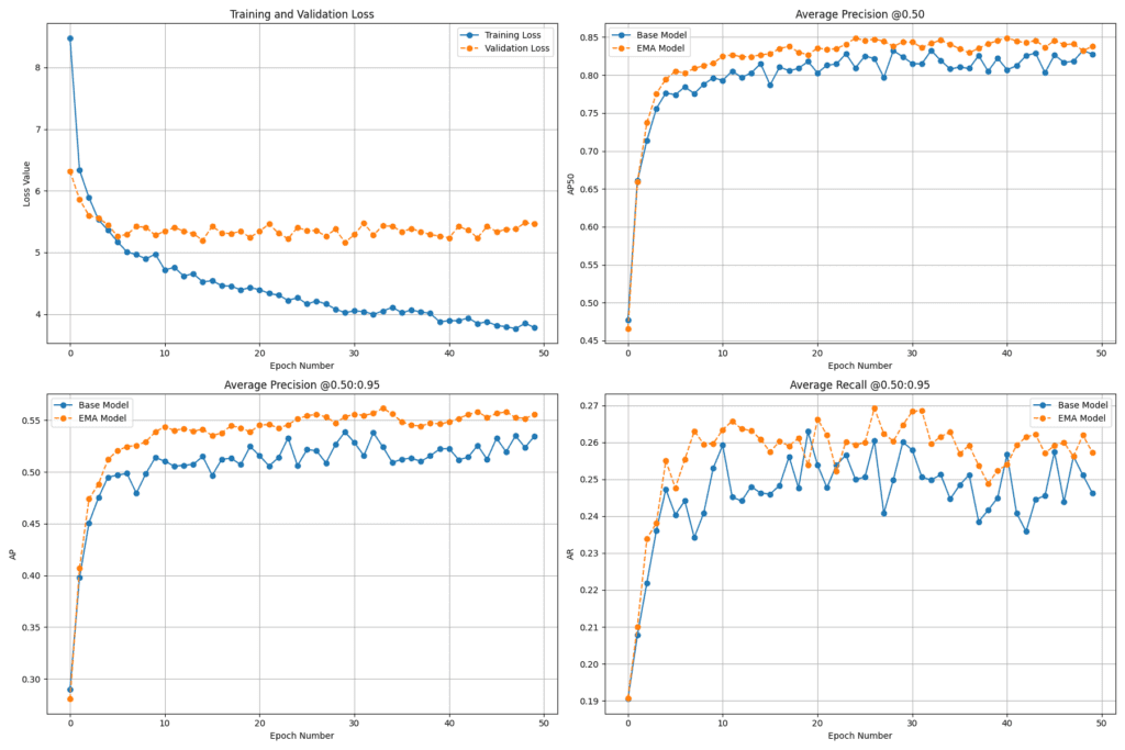
To assess the performance of the fine-tuned RF-DETR model on the aquatic dataset, we plotted key evaluation metrics over 50 training epochs. This metrics graph provide valuable insights into the model’s learning behavior, accuracy, and generalization performance. The plots compare the Base Model with an Exponential Moving Average (EMA) Model, which helps stabilize training and often leads to better generalization.
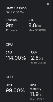
Before concluding the blog, below image demonstrates the consumption of CPU/GPU during fine-tuning training. We performed all our experiments on Kaggle Platform utilizing P100 GPUs.
Key Takeaways
- RF-DETR is a real-time object detection model developed by Roboflow that builds upon the strengths of Deformable DETR and LW-DETR while integrating the DINOv2 backbone for superior domain adaptability.
- The model eliminates the need for traditional detection components like anchor boxes and NMS, leveraging transformer-based architecture for end-to-end object detection.
- Two model variants—Base (29M) and Large (128M)—offer flexibility between speed and accuracy, making RF-DETR suitable for edge deployments and high-performance scenarios.
- The Supervision library by Roboflow simplified the entire training and visualization workflow.
- The model can be effectively fine-tuned for specific domains, as demonstrated with the aquatic dataset, leveraging its pre-trained knowledge.
Conclusion
RF-DETR proves to be a versatile and high-performing model for real-time object detection across general and domain-specific tasks. Its robust architecture, powered by transformer-based architectures like Deformable DETR and LW-DETR and pre-trained backbones like DINOv2, makes it a good choice for developers working on custom detection problems.
By combining RF-DETR with powerful tools like Supervision, AI enthusiasts can quickly build high-quality, production-ready models that adapt well to novel domains. Whether you’re deploying on the edge or experimenting in research, RF-DETR offers the flexibility and performance to push your computer vision projects forward.



100K+ Learners
Join Free OpenCV Bootcamp3 Hours of Learning