Robotics, once a specialized and niche field, has surged into the mainstream with the rapid development of autonomous vehicles, quadruped robots, and humanoids. What’s fueling this revolution? The drive to automate repetitive tasks and free up human ingenuity for more complex problem-solving. As Agility Robotics puts it, the goal is to “Build robot partners that augment the human workforce, ultimately enabling humans to be more human.” At the core of many robotic systems, including autonomous vehicles, is the PID controller, which plays a crucial role in achieving precision and stability in automated processes.
Many robots in the world today aren’t fully autonomous; instead, they are only partially automated, relying heavily on structured environments and controlled conditions. These kinds of robots are hardware heavy, and have very little software contributions. But, when it comes to fully automated systems, the real challenge shifts to software. No doubt it’s a big challenge to design the hardware for a humanoid or quadruped robot, as it must closely align with the control systems, like gait patterns. However the software is more prone to failure and presents more critical challenges. Let’s step toward learning robotics software development and its key components.
This is the sixth article in the robotics series. So far, we’ve covered perception and computer vision topics like LiDAR SLAM methods (LOAM, LeGO-LOAM), explored Monocular SLAM with OpenCV Python, provided a ROS 2 and Carla setup guide, and discussed the internals of ROS 2. In this article, we’ll start the final project: Building a 6DoF Autonomous Vehicle for Static Obstacle Avoidance Using ROS 2 and Carla. Initially, we’ll focus on the basics.
- Understand and implement PID controller
- Moving a vehicle on CARLA using PID Controller, based on a set of waypoints generated from the start and end pose
- Integrate the workflow with ROS 2
NB:
- We’ll primarily write the code in Python to keep things easy to understand and majorly focus on system design.
- If you don’t have the CARLA and ROS 2 installed its advice to follow this ROS 2 CARLA setup guide for Ubuntu 20.04.
- Robotics Software Development
- What are P, PI and PID Controller ?
- Proportional (P) Controller
- Proportional-Integral (PI) Controller
- Proportional-Integral-Derivative (PID) Controller
- Introduction to Lateral Control
- CARLA ROS2 Integration
- Key Takeaways
- Conclusion
- References
Robotics Software Development
Robotics is a multidisciplinary field involving mechanical design and various areas of computer science, such as computer architecture, networking, and databases. It is often seen as system engineering due, to its integration of different domains. The core software components in robotics are mathematically intensive and must be highly optimized to maintain low latency. The major software components of robotics are:
- Perception
- Planning
- Control
A general autonomous stack irrespective of its environment will look like this (see below image), well at least in its initial iterations. The stack consists of 4 sub stacks, the sensor stack, perception stack, planning and control stack. The sensor stack consists of two cameras, front and rear, along with a LiDAR on top of the vehicle. The perception stack consists of Localization and Mapping (we have been talking about this throughout the series), HD-Maps are also very important for navigation, but there have been approaches proposed to create HD-Maps on-the-fly and finally Object detection and segmentation used for detecting landmarks and understanding drivable area.
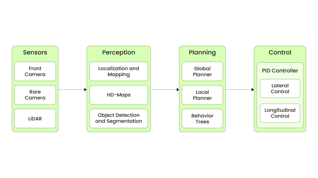
The planning module is divided into three parts. It is known that having a global and local planner might suffice for many use cases, but when it comes to handling different scenarios, a robot needs to have a behavior tree in place. Let’s take the example of an autonomous vehicle. There can be scenarios like following traffic lights, parking, or off-road driving, where different planners are needed for different tasks. And finally, the controls—generally, a well-tuned PID controller is used for actuator signals. It is typically divided into two steps: lateral control for waypoint following and longitudinal control for velocity management. In this article, we will explore the control part in more detail.
If we were to design a basic autonomous vehicle in CARLA, how would we do that? Emphasizing “in CARLA” since it will be inside the simulator makes it much easier to work in a structured environment. Additionally, we can leverage all the API goodness provided by CARLA to get a lot of pre-computed estimates. The system architecture below shows how CARLA and ROS 2 are used to create autonomous path-following vehicles.
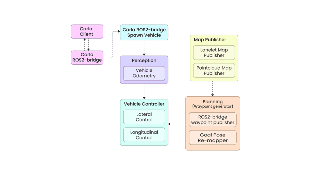
We begin by starting the CARLA client and the CARLA ROS bridge. These two modules communicate to send data from CARLA to ROS 2. Initially, this will provide information about the CARLA world, weather, and status. Next, the CARLA ros-bridge spawn vehicle node needs to be started to spawn a vehicle in the CARLA world, which will provide a lot of information about the vehicle, sensor data, and traffic through ROS 2 topics. After that, the Lanelet and Point Cloud maps are launched, giving us a view of the drivable area.
The Lanelet map and point cloud map gives an understanding about the surroundings and drivable areas. After that’s known to us, we can then launch the waypoint generator. It takes the vehicle’s starting and goal locations to generate the shortest path, which is composed of waypoints. Waypoints are essentially a series of 3D points that define the global path. The vehicle’s task is to follow these waypoints to reach its goal. To achieve this, a PID controller is used, which takes the waypoint coordinates and the vehicle’s odometry (current position and orientation at each timestamp) to generate the actuator signals. The odometry data also comes from CARLA.
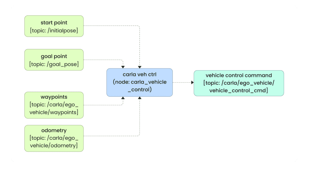
From the ROS 2 perspective, the system works like this: carla vehicle ctrl node is the centerpiece of the workflow. It subscribes to the start and end positions topic, along with the generated waypoints for the vehicle to follow, and uses the vehicle’s odometry to compute the control commands. The topic /carla/ego_vehicle/vehicle_control_cmd receives these control commands and moves the vehicle. The entire system is visualized in RViz2.
Simple, right? Looking ahead, the future scope of this blog will involve implementing proper perception and planning tasks, as shown in Figure 1. However, for now, we’ll be using CARLA’s perception and planning data.
As CARLA already handles the odometry and planning, we’ll primarily focus on vehicle control. For this, we’ve decided to use a PID controller, though more advanced controllers could be explored. Below are the topics we will cover:
- What are P, PI and PID Controllers?
- Implement PID control python.
- What is Longitudinal Control and Lateral Control?
What are P, PI and PID Controller ?
As mentioned, we will use a PID controller to move the vehicle along a desired trajectory by generating the necessary actuator signals. But before that what does “actuator signals” actually mean? Actuators are the parts of a robot that convert electrical energy into physical movement, typically motors or hydraulics found in the robot’s joints. The controller’s job is to generate the right amount of electrical energy to achieve the desired movement. For example, if you have a vehicle and want it to travel from one place to another, or if you have a robotic arm and want it to grab an apple from a table, the planner gives you the desired physical movement — it can be represented either as a velocity profile, a trajectory, or both. It’s the controller’s job to follow the proposed path.
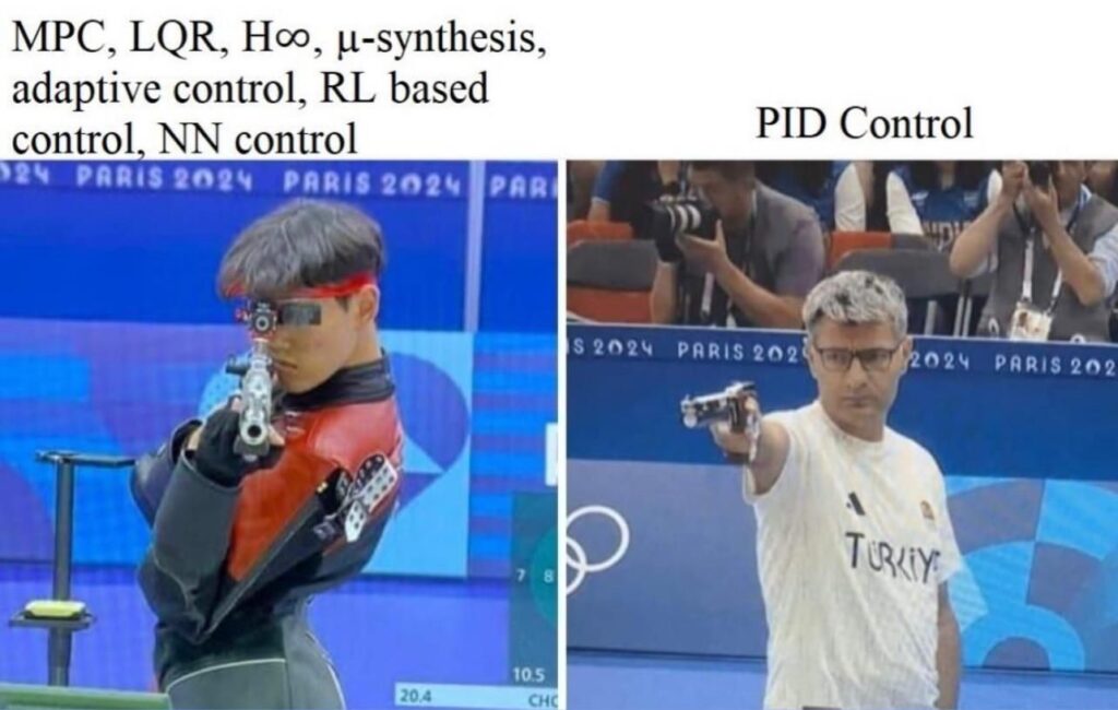
Now that we understand the purpose let’s explore how the controller does that. There are different kinds of controllers available such as PID controller, Fuzzy Logic Controllers, Model Predictive control (MPC), Non-linear Model Predictive control (NLMPC), Neural Network Controllers, RL based controllers etc. But in this article we will be focusing on the PID controller which is one of the most simple but efficient controllers. And legends have it that a properly tuned PID controller can still give all the modern controllers a run for the money. Despite being one of the oldest controller methods (more than 100 years) it is still used in industry and academia.
P, I, and D in a PID controller stand for proportional, integral, and derivative, respectively. Each term contributes to controlling a robot. Let’s break it down with an example: Say you have an autonomous vehicle and want to travel from home to your office while maintaining a velocity of 50 m/s. Driving a vehicle autonomously at a constant velocity is an Advanced Driver Assistance System (ADAS) feature known as Cruise Control.
From a control perspective, the goal is to achieve this by continuously adjusting the throttle based on the difference between the current vehicle speed and the target speed. Diagrammatically, it can be represented as follows:
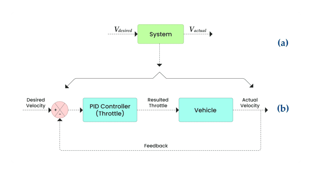
At a high level, you can think of it as a system where you provide the desired velocity, and it returns the system response— the actual velocity (see the above figure a). The controller’s goal is to make the actual velocity equal to the desired velocity, meaning the difference between them should eventually reach zero.
If we zoom into the system (from figure a), you’ll see (figure b) the controller and the vehicle (as the process/plant). Here, the controller’s job is to take the desired velocity and the actual velocity as input and compute the difference between them to produce a throttle value. Providing the vehicle’s response to the PID controller is called closed-loop feedback.
Now that we have an overall understanding of what PID controllers are doing, let’s entangle PID controllers and understand the contributions of P,I and D terms.
Proportional (P) Controller
The P controller addresses the difference between the current and desired velocity. For example, if the current velocity is 0 and the target is 50 m/s, the throttle needs to be increased to close that gap. The larger the error, the more throttle is applied, meaning the throttle is proportional to the error, represented as:
![]()
![]()
Mathematically this can be written as,
![]() , Here,
, Here, ![]() , is proportional gain.
, is proportional gain.
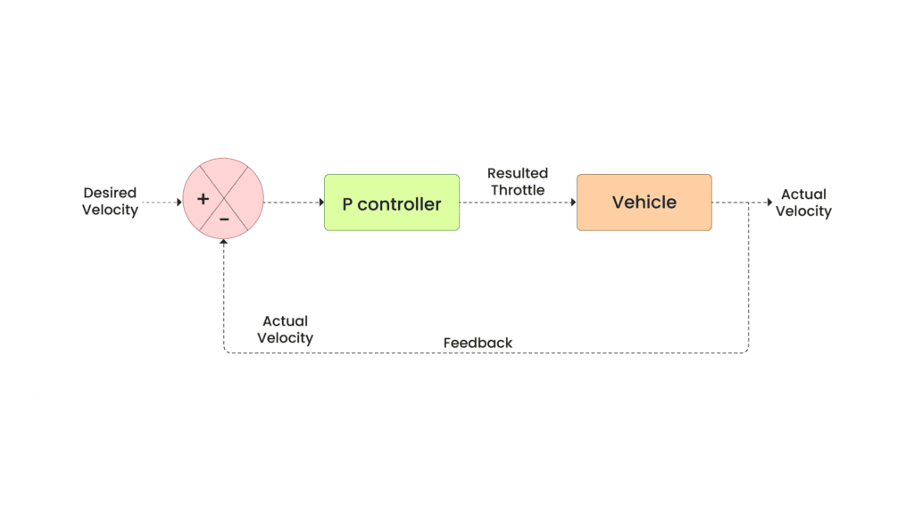
The block diagram below represents a Proportional (P) controller used in a feedback control system to regulate the velocity of a vehicle. The desired velocity is input into the system and compared with the actual velocity to determine the error. This error is fed into the P controller, which adjusts the throttle of the vehicle based on the proportional gain of the error. The output is the actual velocity of the vehicle, which is feedback into the system for continuous adjustments, maintaining the desired velocity. The loop is closed with feedback, ensuring real-time correction of the vehicle’s velocity.
Below is the python code for simple P controller,
import numpy as np
import matplotlib.pyplot as plt
from matplotlib.widgets import Slider

# Define PID Controller class with resistance
class PIDControllerWithResistance:
    def __init__(self, Kp, set_point=0, resistance_factor=0.1):
        self.Kp = Kp
        self.set_point = set_point
        self.resistance_factor = resistance_factor  # Resistance to throttle (e.g., air resistance, friction)

    def update(self, current_value, dt):
        # Apply the same PID control logic but factor in resistance
        error = self.set_point - current_value
        output = self.Kp * error
        return output - self.resistance_factor * current_value  # Reduce output by a resistance factor

# Simulation parameters
dt = 0.1  # Time step
time = np.arange(0, 50, dt)  # Simulation time

# Initialize the PID controller with disturbance (resistance)
pid_with_resistance = PIDControllerWithResistance(Kp=1.0, set_point=50, resistance_factor=0.2)

# Initial conditions
speed = 0
throttle_with_resistance = []
speed_record_with_resistance = []

# Simulate the system with resistance
for t in time:
    control = pid_with_resistance.update(speed, dt)
    speed += control * dt  # Speed is affected by throttle control and resistance
    throttle_with_resistance.append(control)
    speed_record_with_resistance.append(speed)

# Plot setup
fig, ax = plt.subplots()
plt.subplots_adjust(left=0.1, bottom=0.3)

l, = plt.plot(time, speed_record_with_resistance, label="Speed Output (With Resistance)")
plt.axhline(pid_with_resistance.set_point, color='r', linestyle='--', label='Set Point')
plt.xlabel('Time [s]')
plt.ylabel('Speed [m/s]')
plt.title('PID Cruise Control with Resistance')
plt.legend()
plt.show()
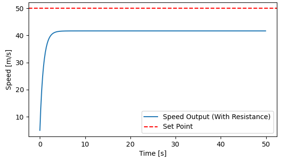
Result:
There are a few assumptions this code makes:
- We assume the relationship between throttle and vehicle velocity is linear, meaning increasing the throttle increases the velocity. That’s why we simply do
speed += control * dt. By multiplying thecontrolbydt, we ensure the speed changes incrementally over each small time interval, simulating a gradual change. - For simplicity, we assume that resistance is linearly proportional to speed in this model.
We first define the PIDControllerWithResistance class, which takes the ![]() value, set-point, and resistance value. In the update function, we calculate the error as
value, set-point, and resistance value. In the update function, we calculate the error as self.set_point - current_value and multiply it by ![]() to get the throttle. We also include
to get the throttle. We also include output - self.resistance_factor * current_value.
- Multiplying the resistance factor by the current speed (
current_value) creates a more realistic model where resistance increases with speed. - By subtracting this resistance component from the output throttle value, we simulate the need for more throttle to maintain higher speeds, making it harder for the vehicle to accelerate at higher speeds.
We loop through the time-stamp from 0 to 50, keeping dt as 0.1, and call the controller’s update function to get the resulting velocity. However, as you can see, using proportional control alone is insufficient. Although the velocity approaches the set-point, it never fully reaches it. This difference between the steady state and the set-point is called Steady State Error. At this point, the error becomes so small that even multiplying it by ![]() results in minimal change, leaving the velocity almost unchanged.
results in minimal change, leaving the velocity almost unchanged.
Proportional-Integral (PI) Controller
As we can see, the response velocity gets close to the set-point but doesn’t quite reach it. To address this, we can add an Integral controller alongside the Proportional controller. The Integral controller looks at past errors and accumulates them over time. This accumulation of positive error helps push the response closer to the set-point.
Mathematically this can be written as,
![]()
In the below image the Integral (I) controller is added to the parallel of the Proportional (P) controller for regulating the velocity of a vehicle. The desired velocity is compared with the actual velocity to calculate the error. This error is fed into both the controllers: the Proportional (P) controller, which responds proportionally to the current error, and the Integral (I) controller, which considers the cumulative sum of past errors. The outputs from both controllers are summed to adjust the vehicle’s throttle. The actual velocity is then fed back into the system to continuously correct and maintain the desired velocity. This feedback loop allows for more accurate control, especially when compensating for steady-state errors.
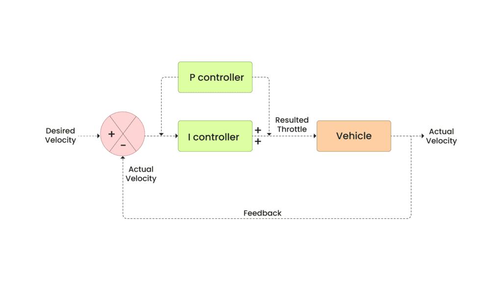
However, a constant increase in the error might cause the Integral controller to overshoot the velocity value, leading to a negative error. When this negative error is summed, it lowers the output of the integrator, resulting in a reduced velocity. That’s why there is an oscillation that’s being created when you plot the response. This is not the expected behaviour.
Below is the code of PI controller using python,
import numpy as np
import matplotlib.pyplot as plt
from matplotlib.widgets import Slider

# Define PID Controller class with resistance
class PIDControllerWithResistance:
    def __init__(self, Kp, Ki, set_point=0, resistance_factor=0.1):
        self.Kp = Kp
        self.Ki = Ki
        self.set_point = set_point
        self.integral = 0
        self.resistance_factor = resistance_factor  # Resistance to throttle (e.g., air resistance, friction)

    def update(self, current_value, dt):
        # Apply the same PID control logic but factor in resistance
        error = self.set_point - current_value
        self.integral += error * dt
        output = self.Kp * error + self.Ki * self.integral
        return output - self.resistance_factor * current_value  # Reduce output by a resistance factor

# Simulation parameters
dt = 0.1  # Time step
time = np.arange(0, 50, dt)  # Simulation time

# Initialize the PID controller with disturbance (resistance)
pid_with_resistance = PIDControllerWithResistance(Kp=1.0, Ki=0.05, set_point=50, resistance_factor=0.05)

# Initial conditions
speed = 0
throttle_with_resistance = []
speed_record_with_resistance = []

# Simulate the system with resistance
for t in time:
    control = pid_with_resistance.update(speed, dt)
    speed += control * dt  # Speed is affected by throttle control and resistance
    throttle_with_resistance.append(control)
    speed_record_with_resistance.append(speed)

# Plot setup
fig, ax = plt.subplots()
plt.subplots_adjust(left=0.1, bottom=0.3)

l, = plt.plot(time, speed_record_with_resistance, label="Velocity Output (With Resistance)")
plt.axhline(pid_with_resistance.set_point, color='r', linestyle='--', label='Set Point')
plt.xlabel('Time [s]')
plt.ylabel('Velocity [m/s]')
plt.title('PID Cruise Control with Resistance')
plt.legend()
plt.show()
Output:
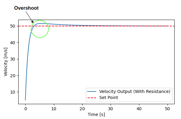
Above code is very similar to the P-controller; we just computer the integral error self.integral += error * dt and add self.Ki * self.integral with the p-controller output. The velocity overshoot is marked using the green circle.
Proportional-Integral-Derivative (PID) Controller
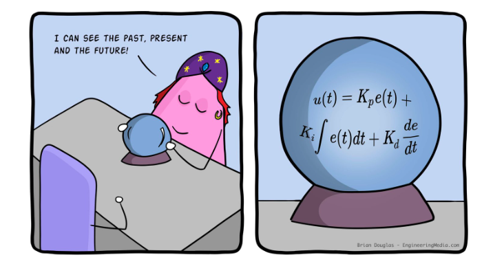
We’re almost there—now, we just need to address the overshoot issue. Typically, the derivative term is added to the PI controller output to dampen the response. The derivative term represents the rate of change of error over time, which intuitively acts as a damping factor. When you add the rate of change of error to the PI controller output, it helps reduce the overshoot. Philosophically, you could say the derivative term “looks into the future” by estimating the change in error and adjusting the PI output accordingly, resulting in a more stable response. Mathematically, it’s represented as:
![]()
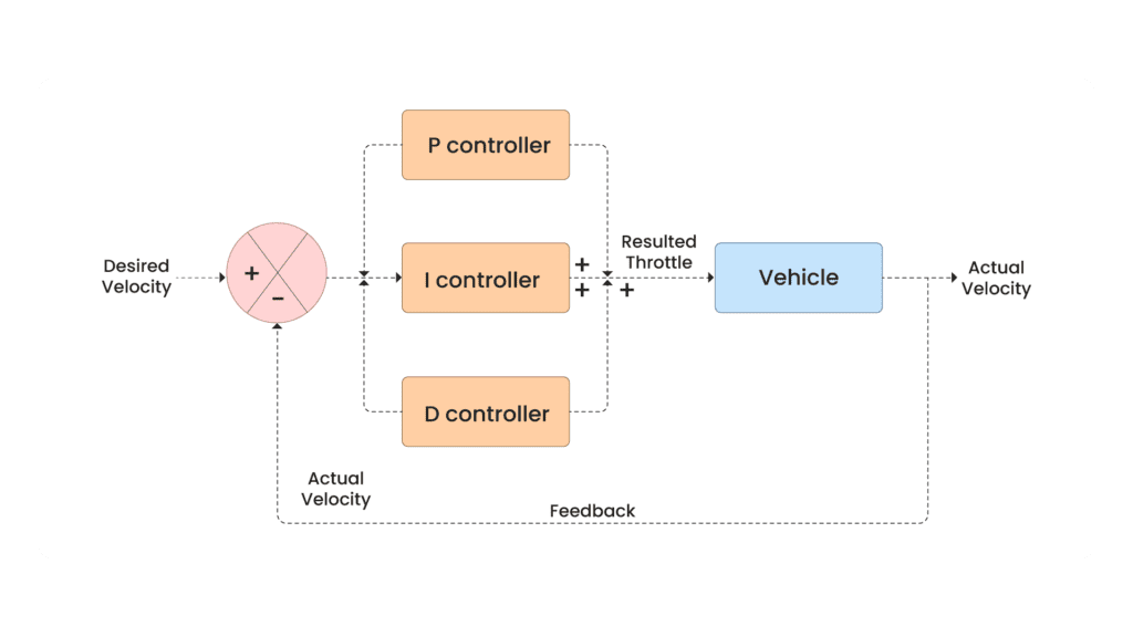
The Derivative (D) controller has now been added in parallel to the PI controller, forming a Proportional-Integral-Derivative (PID) controller. This system is used in a feedback loop to regulate the velocity of a vehicle, enhancing precision by considering the present, past, and predicted future errors. The desired velocity is compared with the actual velocity to compute the error. This error is fed into three controllers: the Proportional (P) controller, which reacts to the current error, the Integral (I) controller, which accounts for the accumulated error over time, and the Derivative (D) controller, which predicts future errors by considering the rate of change of the error. The outputs of these controllers are combined to adjust the vehicle’s throttle, and the actual velocity is fed back into the system for continuous correction, ensuring the desired velocity is maintained with improved precision and stability.
The equation is written with discrete time in mind. The values of ![]() ,
, ![]() , and
, and ![]() are typically found through trial and error, although some algorithms are available to tune the gain values.
are typically found through trial and error, although some algorithms are available to tune the gain values. ![]() represents the derivative gain.
represents the derivative gain.
Below is the python code for PID controller,
import numpy as np
import matplotlib.pyplot as plt
from matplotlib.widgets import Slider

# Define PID Controller class with resistance
class PIDControllerWithResistance:
    def __init__(self, Kp, Ki, Kd, set_point=0, resistance_factor=0.1):
        self.Kp = Kp
        self.Ki = Ki
        self.Kd = Kd
        self.set_point = set_point
        self.prev_error = 0
        self.integral = 0
        self.resistance_factor = resistance_factor  # Resistance to throttle (e.g., air resistance, friction)

    def update(self, current_value, dt):
        # Apply the same PID control logic but factor in resistance
        error = self.set_point - current_value
        self.integral += error * dt
        derivative = (error - self.prev_error) / dt
        output = self.Kp * error + self.Ki * self.integral + self.Kd * derivative
        self.prev_error = error
        return output - self.resistance_factor * current_value  # Reduce output by a resistance factor

# Simulation parameters
dt = 0.1  # Time step
time = np.arange(0, 50, dt)  # Simulation time

# Initialize the PID controller with disturbance (resistance)
pid_with_resistance = PIDControllerWithResistance(Kp=1.0, Ki=0.05, Kd=0.01, set_point=50, resistance_factor=0.05)

# Initial conditions
speed = 0
throttle_with_resistance = []
speed_record_with_resistance = []

# Simulate the system with resistance
for t in time:
    control = pid_with_resistance.update(speed, dt)
    speed += control * dt  # Speed is affected by throttle control and resistance
    throttle_with_resistance.append(control)
    speed_record_with_resistance.append(speed)

# Plot setup
fig, ax = plt.subplots()
plt.subplots_adjust(left=0.1, bottom=0.3)

l, = plt.plot(time, speed_record_with_resistance, label="Velocity Output (With Resistance)")
plt.axhline(pid_with_resistance.set_point, color='r', linestyle='--', label='Set Point')
plt.xlabel('Time [s]')
plt.ylabel('Velocity [m/s]')
plt.title('PID Cruise Control with Resistance')
plt.legend()
plt.show()
Result:
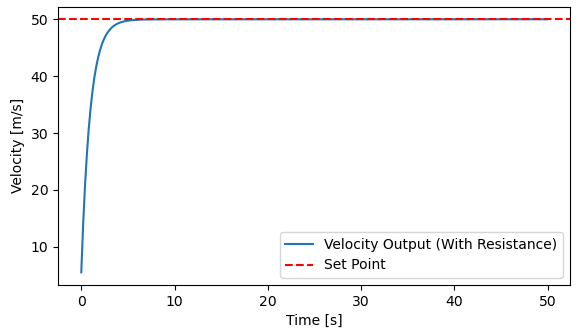
The code is very similar to the PI controller code, with the addition of the derivative term to the PI controller output. It is calculated as derivative = (error - self.prev_error) / dt.
To summarize the PID controller, P looks at the present error, I looks at the past errors, and D anticipates future errors. Together, they regulate the output response to achieve the desired result.
Introduction to Lateral Control
When it comes to moving a robot from one position to another, using only velocity control (commonly referred to as Longitudinal Control) is insufficient for ensuring accurate path following. While longitudinal control governs the speed of the robot, a planner typically generates a trajectory consisting of 3D waypoints from the robot’s current position to the goal. To follow this trajectory effectively, the robot also requires lateral control, which adjusts its steering angle or orientation to maintain the desired path. Lateral control is crucial for handling deviations, ensuring smooth navigation, and achieving precise positioning, especially when moving through complex environments.
There are various types of lateral controllers designed to handle this task, each suited to different applications and conditions. These can be broadly categorized into geometric and dynamic controllers.
- Geometric controller:
- Pure Pursuit (carrot following)
- Stanley
- PID
- Dynamic controller:
- MPC controller
- Other control systems
- sliding mode, feedback linearization etc.
We will be using PID for lateral control but you can experiment with these controllers for better maneuvers.
CARLA ROS2 Integration
Now that we understand the PID controller, let’s use it to move our vehicle in CARLA. There are only two main files that are used to do this, vehicle_ctrl.py and lat_lon_ctrl.py; we will go through them one by one.
First understand the Longitudinal and lateral control code in the lat_lon_ctrl.py. The below code is taken from CARLA itself, with slight modifications.
""" This module contains PID controllers to perform lateral and longitudinal control. """

from collections import deque
import math
import numpy as np
import carla
from agents.tools.misc import get_speed

...

class PIDLongitudinalController():
    """
    PIDLongitudinalController implements longitudinal control using a PID.
    """

    def __init__(self, vehicle, K_P=1.0, K_I=0.0, K_D=0.0, dt=0.03):
        """
        Constructor method.

            :param vehicle: actor to apply to local planner logic onto
            :param K_P: Proportional term
            :param K_D: Differential term
            :param K_I: Integral term
            :param dt: time differential in seconds
        """
        self._vehicle = vehicle
        self._k_p = K_P
        self._k_i = K_I
        self._k_d = K_D
        self._dt = dt
        self._error_buffer = deque(maxlen=10)

    def run_step(self, target_speed, debug=False):
        """
        Execute one step of longitudinal control to reach a given target speed.

            :param target_speed: target speed in Km/h
            :param debug: boolean for debugging
            :return: throttle control
        """
        current_speed = get_speed(self._vehicle)

        if debug:
            print('Current speed = {}'.format(current_speed))

        return self._pid_control(target_speed, current_speed)

    def _pid_control(self, target_speed, current_speed):
        """
        Estimate the throttle/brake of the vehicle based on the PID equations

            :param target_speed:  target speed in Km/h
            :param current_speed: current speed of the vehicle in Km/h
            :return: throttle/brake control
        """

        error = target_speed - current_speed
        self._error_buffer.append(error)

        if len(self._error_buffer) >= 2:
            _de = (self._error_buffer[-1] - self._error_buffer[-2]) / self._dt
            _ie = sum(self._error_buffer) * self._dt
        else:
            _de = 0.0
            _ie = 0.0

        return np.clip((self._k_p * error) + (self._k_d * _de) + (self._k_i * _ie), -1.0, 1.0)

    def change_parameters(self, K_P, K_I, K_D, dt):
        """Changes the PID parameters"""
        self._k_p = K_P
        self._k_i = K_I
        self._k_d = K_D
        self._dt = dt


class PIDLateralController():
    """
    PIDLateralController implements lateral control using a PID.
    """

    def __init__(self, vehicle, offset=0, K_P=1.0, K_I=0.0, K_D=0.0, dt=0.03):
        """
        Constructor method.

            :param vehicle: actor to apply to local planner logic onto
            :param offset: distance to the center line. If might cause issues if the value
                is large enough to make the vehicle invade other lanes.
            :param K_P: Proportional term
            :param K_D: Differential term
            :param K_I: Integral term
            :param dt: time differential in seconds
        """
        self._vehicle = vehicle
        self._k_p = K_P
        self._k_i = K_I
        self._k_d = K_D
        self._dt = dt
        self._offset = offset
        self._e_buffer = deque(maxlen=10)

    def run_step(self, waypoint):
        """
        Execute one step of lateral control to steer
        the vehicle towards a certain waypoin.

            :param waypoint: target waypoint
            :return: steering control in the range [-1, 1] where:
            -1 maximum steering to left
            +1 maximum steering to right
        """
        return self._pid_control(waypoint, self._vehicle.get_transform())

    def _pid_control(self, waypoint, vehicle_transform):
        """
        Estimate the steering angle of the vehicle based on the PID equations

            :param waypoint: target waypoint
            :param vehicle_transform: current transform of the vehicle
            :return: steering control in the range [-1, 1]
        """
        # Get the ego's location and forward vector
        ego_loc = vehicle_transform.location
        v_vec = vehicle_transform.get_forward_vector()
        v_vec = np.array([v_vec.x, v_vec.y, 0.0])

        # Get the vector vehicle-target_wp
        if self._offset != 0:
            # Displace the wp to the side
            w_tran = waypoint
            r_vec = w_tran.get_right_vector()
            w_loc = w_tran.location + carla.Location(x=self._offset*r_vec.x,
                                                         y=self._offset*r_vec.y)
        else:
            w_loc = waypoint.location

        w_vec = np.array([w_loc.x - ego_loc.x,
                          w_loc.y - ego_loc.y,
                          0.0])

        wv_linalg = np.linalg.norm(w_vec) * np.linalg.norm(v_vec)
        if wv_linalg == 0:
            _dot = 1
        else:
            _dot = math.acos(np.clip(np.dot(w_vec, v_vec) / (wv_linalg), -1.0, 1.0))
        _cross = np.cross(v_vec, w_vec)
        if _cross[2] < 0:
            _dot *= -1.0

        self._e_buffer.append(_dot)
        if len(self._e_buffer) >= 2:
            _de = (self._e_buffer[-1] - self._e_buffer[-2]) / self._dt
            _ie = sum(self._e_buffer) * self._dt
        else:
            _de = 0.0
            _ie = 0.0

        return np.clip((self._k_p * _dot) + (self._k_d * _de) + (self._k_i * _ie), -1.0, 1.0)

    def change_parameters(self, K_P, K_I, K_D, dt):
        """Changes the PID parameters"""
        self._k_p = K_P
        self._k_i = K_I
        self._k_d = K_D
        self._dt = dt
Longitudinal Control
PIDLongitudinalController class contains the code for longitudinal control, we first initialize the PID gains, carla vehicle instance and the error buffer (used for d-control). run_step is the function that calls the _pid_control function for the PID updates iteratively from an external function. The real magic is inside the _pid_control function. The implementation is very simple and similar to the PID implementation above. We first calculate the error, error = target_speed - current_speed populate the self._error_buffer list. If self._error_buffer has more than 2 elements then we calculate the derivative error (_de) and integral error (_ie) and finally return the total control output as np.clip((self._k_p * error) + (self._k_d * _de) + (self._k_i * _ie), -1.0, 1.0), by clipping it from -1 to 1.
Lateral Control
Lateral control is a bit tricky. Let’s go through how the lateral error is calculated before jumping in the code. The error is formulated as the signed angle between the vehicle’s forward vector and the waypoint vector. The sign of the angle is decided based on whether the vehicle is to the left or right of the desired path. Angle should be positive (to the right) or negative (to the left).
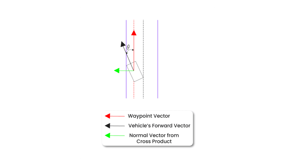
In lateral control for autonomous vehicles, the main goal is to keep the vehicle on the correct trajectory or path. The vehicle’s lateral control is typically concerned with minimizing the deviation from this desired path, which is achieved by controlling the steering angle. The code you provided uses a PID (Proportional, Integral, Derivative) controller to adjust the vehicle’s steering angle based on this deviation.
Let’s go through the code. PIDLateralController is where the lateral control is defined. Below is how the error angle is calculated,
1. Vehicle’s Forward Vector (v_vec):
The forward vector represents the direction in which the vehicle is currently moving, derived from the vehicle’s transform (vehicle_transform.get_forward_vector()). It is a 3D vector, but only the x and y components are used since the vehicle is moving on a 2D plane.

2. Waypoint Vector (w_vec):
The waypoint vector represents the direction from the vehicle’s current position (ego_loc) to the target waypoint (w_loc):

3. Dot Product and Angle:
The error between the vehicle’s heading and the target waypoint is measured by the angle between the vehicle’s forward vector and the waypoint vector. This is calculated using the dot product and the magnitudes of these vectors:
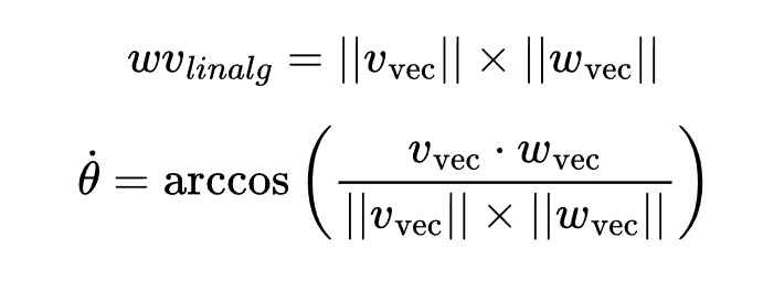
This angle (_dot) represents the lateral error in radians.
4. Cross Product for Sign:
To determine whether the vehicle is to the left or right of the desired path (i.e., the sign of the error), the cross product between the forward vector and waypoint vector is calculated:

The sign of the third component of the cross product (z-component) determines whether the angle should be positive (to the right) or negative (to the left). If the z-component is negative, the angle is inverted:

Thus, the lateral error (_dot) is a signed angle representing how much the vehicle needs to steer to align itself with the waypoint.
PID Control Application
The error (_dot) is passed into the PID controller, which uses the following equation:

Where:
 is the proportional gain.
 is the integral gain (which sums up the past errors to reduce steady-state error).
 is the derivative gain (which responds to changes in the error to dampen oscillations).
 is the current angular error (from the dot product calculation).
 is the accumulated error over time.
 is the rate of change of the error.
Now that we are done with PID control, let’s see how we will run it with ROS 2.
Now let’s go through the vehicle_ctrl.py.
class CarlaVehicleControl(Node):
    def __init__(self):
        super().__init__('carla_route_planner')


        # Subscribers
        self.initialpose_sub = self.create_subscription(
            PoseWithCovarianceStamped,
            '/initialpose',
            self.initialpose_callback,
            10
        )
        self.goal_pose_sub = self.create_subscription(
            PoseStamped,
            '/goal_pose',
            self.goal_pose_callback,
            10
        )
        self.waypt_sub = self.create_subscription(
            Path,
            '/carla/ego_vehicle/waypoints',
            self.waypoints_callback,
            10
        )
        # Subscriber to the /carla/ego_vehicle/odometry topic
        self.odom_sub = self.create_subscription(
            Odometry,
            '/carla/ego_vehicle/odometry',
            self.odometry_callback,
            10)


        self.vehicle_control_publisher = self.create_publisher(CarlaEgoVehicleControl,
                                                      '/carla/ego_vehicle/vehicle_control_cmd',
                                                      10)

        # Initialize Carla client and map
        self.client = Client('localhost', 2000)
        self.client.set_timeout(10.0)

        # Get the current world
        self.world = self.client.get_world()


        # Check if Town01 is already loaded
        if 'Town01' not in self.world.get_map().name:
            print("Town01 is not loaded. Loading Town01...")
            self.world = self.client.load_world('Town01')
            print("Done!")
        else:
            print("Town01 is already loaded.")


        self.map = self.world.get_map()
        # Initialize GlobalRoutePlanner
        self.route_planner = GlobalRoutePlanner(self.map, 2.0)

        # Get all actors (vehicles, pedestrians, etc.) in the world
        self.actors = self.world.get_actors()

        # Filter to get only the vehicles get the 0-th veh as there is only one veh
        self.vehicle = self.actors.filter('vehicle.*')[0]

        # Placeholders for start and end poses
        self.start_pose = None
        self.end_pose = None
        self.waypoints_list = []
        self.odom = None

        # TF2 listener and buffer
        # self.tf_buffer = Buffer()
        # self.tf_listener = TransformListener(self.tf_buffer, self)
        # self.vehicle_loc = None

    def odometry_callback(self, msg):


        self.get_logger().info(f"Received odometry data: {msg.pose.pose.position.x}, {msg.pose.pose.position.y}, {msg.pose.pose.position.z}")

        # Extract position and orientation from Odometry message
        x = msg.pose.pose.position.x
        y = -msg.pose.pose.position.y
        z = msg.pose.pose.position.z

        print(" ^^^^ ODOM XYZ: ", x,y,z )

        orientation_q = msg.pose.pose.orientation
        roll, pitch, yaw = euler_from_quaternion(
            [orientation_q.x, orientation_q.y, orientation_q.z, orientation_q.w])

        # Create a carla.Location object
        location = carla.Location(x=x, y=y, z=z)

        # Create a carla.Rotation object
        rotation = carla.Rotation(roll=roll, pitch=pitch, yaw=yaw)

        # Create a carla.Transform object
        transform = carla.Transform(location, rotation)

        self.odom = transform

    def waypoints_callback(self, msg):
        # self.waypoints_list.clear()  # Clear the list before storing new waypoints

        # Iterate through all the waypoints in the Path message
        for pose in msg.poses:
            # Extract the position from the pose
            x = pose.pose.position.x
            y = -pose.pose.position.y
            z = pose.pose.position.z

            # Extract the orientation (quaternion) from the pose
            orientation_q = pose.pose.orientation
            roll, pitch, yaw = euler_from_quaternion(
                [orientation_q.x, orientation_q.y, orientation_q.z, orientation_q.w])

            # Create a carla.Location object
            location = carla.Location(x=x, y=y, z=z)

            # Create a carla.Rotation object
            rotation = carla.Rotation(roll=roll, pitch=pitch, yaw=yaw)

            # Create a carla.Transform object
            transform = carla.Transform(location, rotation)

            # Store the Waypoint in the global list
            self.waypoints_list.append(transform)

            self.get_logger().info(f"Stored {len(self.waypoints_list)} waypoints as carla.libcarla.Waypoint objects.")

    def create_ctrl_msg(self, throttle, steer, brake):
        control_msg = CarlaEgoVehicleControl()
        control_msg.throttle = throttle
        control_msg.steer = steer
        control_msg.brake = brake
        return control_msg

    def initialpose_callback(self, msg):
        self.get_logger().info("Received initialpose")
        self.start_pose = msg.pose.pose

    def goal_pose_callback(self, msg):
        self.get_logger().info("Received goal_pose")
        self.end_pose = msg.pose
        # Clear the waypoints list for the new goal
        self.waypoints_list.clear()
    def get_transform(self, vehicle_location, angle, d=6.4):
        a = math.radians(angle)
        location = carla.Location(
            d * math.cos(a), d * math.sin(a), 2.0) + vehicle_location
        return carla.Transform(location, carla.Rotation(yaw=180 + angle, pitch=-15))

    def setup_PID(self, vehicle):
        """
        This function creates a PID controller for the vehicle passed to it
        """
        args_lateral_dict = {
            'K_P': 0.5,  # Reduced proportional gain for smoother steering
            'K_D': 0.1,  # Small derivative gain to dampen oscillations
            'K_I': 0.01, # Small integral gain to correct for long-term drift
            'dt': 0.05
        }

        args_long_dict = {
            'K_P': 0.2,  # Slightly lower gain for acceleration control
            'K_D': 0.3,  # Moderate derivative gain
            'K_I': 0.01, # Small integral gain
            'dt': 0.05
        }

        PID= VehiclePIDController(vehicle,args_lateral=args_lateral_dict,args_longitudinal=args_long_dict)

        return PID


    def find_dist_veh(self, vehicle_loc,target):
        dist = math.sqrt( (target.location.x - vehicle_loc.x)**2 + \
                         (target.location.y - vehicle_loc.y)**2 )

        return dist


    def drive_through_plan(self, planned_route, vehicle, speed, PID):
        """
        This function drives throught the planned_route with the speed passed in the argument

        """

        i=0
        waypt_cnt = len(planned_route)-1
        target=planned_route[0]

        cnt = 0
        while True:

            self.world.get_spectator().set_transform(self.get_transform(vehicle.get_location() +
                                                                carla.Location(z=1, x=0.5),
                                                                vehicle.get_transform().rotation.yaw-180))

            # vehicle_loc =  vehicle.get_location()
            vehicle_loc =  self.odom.location

            distance_v = self.find_dist_veh(vehicle_loc,target)


            control = PID.run_step(speed,target)
            # vehicle.apply_control(control)
            ctrl_msg = self.create_ctrl_msg(control.throttle,
                                            control.steer,
                                            control.brake)
            self.vehicle_control_publisher.publish(ctrl_msg)

            if i==(len(planned_route)-1):
                print("last waypoint reached")
                break


            if (distance_v<3.5):

                control = PID.run_step(speed,target)
                # vehicle.apply_control(control)
                ctrl_msg = self.create_ctrl_msg(control.throttle,
                            control.steer,
                            control.brake)
                self.vehicle_control_publisher.publish(ctrl_msg)
                i=i+1
                target=planned_route[i]


            if cnt%5==0:
                print("=----------------------------------------------------------")
                print(f"\n{GREEN} ***** from current loc to {i}/{waypt_cnt} waypoint distance: {distance_v}{RESET}\n")
                print("ROS2 vehilce location: ", self.odom.location)
                print("CARLA vehilce location: ", vehicle.get_location())
                print("target location: ", target.location)
                rclpy.spin_once(self)

            # time.sleep(0.1)  # Add a slight delay to reduce control frequency
            # time.sleep(1)  # Add a 1-second delay

            # print("throttle: ", control.throttle)
            cnt+=1

        control = PID.run_step(0,planned_route[len(planned_route)-1])
        # vehicle.apply_control(control)
        ctrl_msg = self.create_ctrl_msg(control.throttle,
                            control.steer,
                            control.brake)
        self.vehicle_control_publisher.publish(ctrl_msg)


    def run(self):
        desired_velocity=10 #Km/h

        while rclpy.ok():
            rclpy.spin_once(self)

            if self.start_pose is None or self.end_pose is None:
                self.get_logger().info(f'Start pose: {self.start_pose}, End pose: {self.end_pose}')

            elif not self.waypoints_list:
                self.get_logger().info('Waiting for waypoints to be generated...')

            else:
                # Delay to ensure waypoints are populated
                self.get_logger().info('Waiting a bit for waypoints to be fully populated...')
                time.sleep(1)  # Add a 1-second delay
                self.get_logger().info(f'Generated {len(self.waypoints_list)} waypoints from start to end pose')


                # calculating life time of the marker
                total_dist = self.find_dist_veh(self.waypoints_list[0].location, self.waypoints_list[len(self.waypoints_list)-1])
                marker_life_time = (total_dist/desired_velocity) * 3.6


                # Draw waypoints on the Carla map
                for w in self.waypoints_list:
                    # print("self.waypoints_list: ",w.location)
                    self.world.debug.draw_string(w.location, 'O', draw_shadow=False,
                                                 color=Color(r=255, g=0, b=0), life_time=5000000.0,
                                                 persistent_lines=True)


                # drive the vehicle
                PID=self.setup_PID(self.vehicle)
                self.drive_through_plan(self.waypoints_list,self.
                                        vehicle,desired_velocity,
                                        PID)


                # After processing, break the loop if needed
                break

def main(args=None):
    rclpy.init(args=args)
    route_planner = CarlaVehicleControl()
    route_planner.run()
    rclpy.shutdown()
If you’ve been following the robotics series, the code above should be easy to understand. The core of the code lies in the run() and drive_through_plan() functions.
- When the main function is called, the callback goes to the
run()function. You’ll notice we’re not usingrclpy.spin(), but insteadrclpy.spin_once(self). This is becauserclpy.spin()continuously spins to collect all the published data. However, we don’t have the luxury of spinning solely for that purpose—we also need to move the vehicle based on the inputs. If we only focus on that, we might miss the published data, causing the vehicle to go out of control and possibly crash into a wall.
This can be handled by either:- Running these two tasks in separate threads.
- Running
rclpy.spin_once()withwhile rclpy.ok()to collect the published data, and while in thedrive_through_planloop, usingrclpy.spin_once()periodically to update the subscriber variable.
- The explanation of how
drive_through_planworks is as follows: it starts by setting a target trajectory point and entering a while loop. This loop continues until the vehicle reaches its goal position. Inside the loop, it first calculates the distance between the vehicle’s location and the target waypoint, then uses the PID controller to calculate the steer and throttle values based on the desired velocity and the target waypoint. These values are applied to the vehicle. This process repeats until the distance between the vehicle and the target waypoint is less than 3.5. At that point, it recalculates the throttle and steer values, applies them, and updates the target waypoint. If the iteration reaches the last waypoint, the vehicle brakes and applies control based on a desired speed of zero. Additionally, in theif cnt%5==0:condition, it executesrclpy.spin_once(self)to update the odometry values.
With everything in place, all that’s left is to run the code and watch it in action.
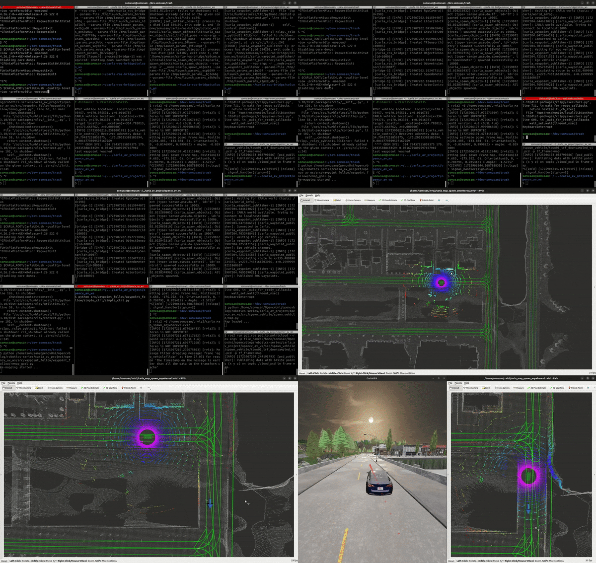
Download the code from below “Download Example Code” button and run the following commands,
# in a new terminal, run carla first
# ./CarlaUE4.sh  # or ./CarlaUE4.sh -prefernvidia # $ ~/carla_simulator/PythonAPI/util/config.py --map Town01
$CARLA_ROOT/CarlaUE4.sh -quality-level=Low -prefernvidia -nosound

# in a new terminal, get inside the `carla-ros-bridge/colcon_ws` folder and source the workspace; launch the `carla ros-bridge`
cd ~/carla-ros-bridge/colcon_ws && source install/setup.bash
ros2 launch carla_ros_bridge carla_ros_bridge.launch.py synchronous_mode:=True town:=Town01 # <town number, eg: 03>


# in a new terminal, launch the objects.json; launch ros-bridge
# cd ~/carla-ros-bridge/colcon_ws
cd ~/carla-ros-bridge/colcon_ws && source install/setup.bash

ros2 launch carla_spawn_objects carla_example_ego_vehicle.launch.py spawn_sensors_only:=False objects_definition_file:=<absolute path to>/src/vehicle_ctrl/vehicle_ctrl/config/objects.json


# load the town1 lanelet map
python src/vehicle_ctrl/vehicle_ctrl/map.py


# in new terminal, launch the rviz2 [set the global frame to map in rviz2]
rviz2 -d /src/vehicle_ctrl/rviz2/carla_map_spawn_anywherev2.rviz


# in a new terminal, get inside the `carla-ros-bridge/colcon_ws` folder and source the workspace; waypoint publisher
cd ~/carla-ros-bridge/colcon_ws && source install/setup.bash
ros2 launch carla_waypoint_publisher carla_waypoint_publisher.launch.py


# goal remap
python src/vehicle_ctrl/vehicle_ctrl/remap_goal.py


# waypoint following using carls ros-bridge
python src/vehicle_ctrl/vehicle_ctrl/simple_ctrl.py
below is a demo on how to run the commands and get the vehicle moving!
Key Takeaways
- Understanding Autonomous Vehicle Architecture: The article breaks down the four essential stacks (sensor, perception, planning, and control) needed for autonomous driving, highlighting how each component contributes to the overall system.
- Real-Time Path Following: Discover how the combination of ROS 2 and CARLA creates an efficient workflow for generating waypoints and controlling vehicle movements in real-time simulations.
- Hands-On Python Code Implementation: The article provides practical Python code examples for implementing PID controllers, making it easier to understand and experiment with real-world robotics applications.
Conclusion
Building an autonomous vehicle in CARLA with ROS 2 and PID control offers an exciting introduction to robotics and autonomous systems. This project highlights the importance of control systems, from longitudinal and lateral movement to real-time feedback loops, while showcasing the power of open-source tools for real-world applications.
By mastering these core concepts, you’ve laid the groundwork for deeper exploration in autonomous technology, such as advanced planners and perception systems. With platforms like ROS 2 and CARLA, the future of robotics is full of possibilities—and now, you’re equipped to be a part of it.
References
- Algorithms for Automated Driving
- Understanding PID Control
- Robot Controllers Part 1: PID (with Dr. Christian Hubicki)
- PID controller Simple explanation with a Quadcopter as example.
- PID Math Demystified





100K+ Learners
Join Free OpenCV Bootcamp3 Hours of Learning