Otsu’s Thresholding Technique

In this post, we will examine Otsu’s method for automatic image thresholding.

What is Image Thresholding?

Image thresholding is used to binarize the image based on pixel intensities. The input to such thresholding algorithm is usually a grayscale image and a threshold. The output is a binary image.

If the intensity of a pixel in the input image is greater than a threshold, the corresponding output pixel is marked as white (foreground), and if the input pixel intensity intensity is less than or equal to the threshold, the output pixel location is marked black (background).

Image thresholding is used in many applications as a pre-processing step. For example, you may use it in medical image processing to reveal tumor in a mammogram or localize a natural disaster in satellite images.

A problem with simple thresholding is that you have to manually specify the threshold value. We can manually check how good a threshold is by trying different values but it is tedious and it may break down in the real world.

So, we need a way to automatically determine the threshold. The Otsu’s technique named after its creator Nobuyuki Otsu is a good example of auto thresholding.

Before we jump into the details of the technique let’s understand how image thresholding relates to image segmentation.

Image Tresholding vs. Image Segmentation

Image segmentation refers to the class of algorithms that partition the image into different segments or groups of pixels.

In that sense, image thresholding is the simplest kind of image segmentation because it partitions the image into two groups of pixels — white for foreground, and black for background.

The figure below shows different types of segmentation algorithms:

segmentation_methods-1 – LearnOpenCV — Pic 1 Highlevel classification of image segmentation approaches

You can see image thresholding (shown using a red bounding box) is a type of image segmentation.

Image thresholding be future sub-divied into the local and global image tresholding algorithms.

In global thresholding, a single threshold is used globally, for the whole image.

In local thresholding, some characteristics of some local image areas (e.g. the local contrast) may be used to choose a different threshold for different parts of the image.

Otsu’s method is a global image thresholding algorithm.

Otsu’s Thresholding Concept

Automatic global thresholding algorithms usually have following steps.

Process the input image
Obtain image histogram (distribution of pixels)
Compute the threshold value $T$
Replace image pixels into white in those regions, where saturation is greater than $T$ and into the black in the opposite cases.

Usually, different algorithms differ in step 3.

Let’s understand the idea behind Otsu’s approach. The method processes image histogram, segmenting the objects by minimization of the variance on each of the classes. Usually, this technique produces the appropriate results for bimodal images. The histogram of such image contains two clearly expressed peaks, which represent different ranges of intensity values.

The core idea is separating the image histogram into two clusters with a threshold defined as a result of minimization the weighted variance of these classes denoted by $\sigma^{2}_w(t)$ .

The whole computation equation can be described as: $\sigma^{2}_w(t) = w_1(t)\sigma^{2}_1(t) + w_2(t)\sigma^{2}_2(t)$ , where $w_1(t), w_2(t)$ are the probabilities of the two classes divided by a threshold $t$ , which value is within the range from 0 to 255 inclusively.

As it was shown in the Otsu’s paper there are actually two options to find the threshold. The first is to minimize the within-class variance defined above $\sigma^{2}_w(t)$ , the second is to maximize the between-class variance using the expression below:
$\sigma^{2}_b(t) = w_1(t)w_2(t)[\mu_1(t)-\mu_2(t)]^{2}$ , where $\mu_i$ is a mean of class $i$ .

The probability $P$ is calculated for each pixel value in two separated clusters $C_1, C_2$ using the cluster probability functions expressed as:
$w_1(t) = \sum_{i=1}^{t}P(i)$ ,
$w_2(t) = \sum_{i=t+1}^{I}P(i)$

It should be noted that the image can presented as intensity function $f(x,y)$ , which values are gray-level. The quantity of the pixels with a specified gray-level $i$ denotes by $i$ . The general number of pixels in the image is $n$ .
Thus, the probability of gray-level $i$ occurrence is:
$P(i) = \frac{n_i}{n}$ .

The pixel intensity values for the $C_1$ are in $[1, t]$ and for $C_2$ are in $[t + 1, I]$ , where $I$ is the maximum pixel value (255).

The next phase is to obtain the means for $C_1, C_2$ , which are denoted by $\mu_1(t), \mu_2(t)$ appropriately:
$\mu_1(t) = \sum_{i=1}^{t}\frac{iP(i)}{w_1(t)}$ ,

$\mu_2(t) = \sum_{i=t+1}^{I}\frac{iP(i)}{w_2(t)}$

Now let’s remember the above equation of the within-classes weighted variance. We will find the rest of its components ( $\sigma_1^{2}, \sigma_2^{2}$ ) mixing all the obtained above ingredients:
$\sigma_1^{2}(t) = \sum_{i=1}^{t}[i - \mu_1(t)]^2 \frac{P(i)}{w_1(t)}$ ,

$\sigma_2^{2}(t) = \sum_{i=t+1}^{I}[i - \mu_2(t)]^2 \frac{P(i)}{w_2(t)}$ .

It should be noted that if the threshold was chosen incorrectly the variance of some class would be large. To get the total variance we simply need to summarize the within class and between-class variances: $\sigma_T^2 = \sigma_w^2(t) + \sigma_b^2(t)$ , where $\sigma_b^2(t) = w_1(t)w_2(t)[\mu_1(t) - \mu_2(t)]^2$ . The total variance of the image ( $\sigma_T^2$ ) does not depend on the threshold.

Thus, the general algorithm’s pipeline for the between-class variance maximization option can be represented in the following way:

calculate the histogram and intensity level probabilities
initialize $w_i(0), \mu_i(0)$
iterate over possible thresholds:
- update the values of $w_i, \mu_i$ , where $w_i$ is a probability and $\mu_i$ is a mean of class $i$
- calculate the between-class variance value $\sigma_b^2(t)$
the final threshold is the maximum $\sigma_b^2(t)$ value

Otsu’s Binarization Application

You could ask what is the real case where Otsu’s approach could be applied? Despite the fact that the method was announced in 1979, it still forms the basis of some complex solutions. Let’s take as an example an urgent task of robotic mapping, concluding in accurate spatial representation of any environment covered by a robot. This information is key for a properly robot autonomous functioning. The non-trivial case is underwater surface mapping described in the article “An improved Otsu threshold segmentation method for underwater simultaneous localization and mapping-based navigation”.

The authors provide improved Otsu’s method as one of the approaches for estimation of the underwater landmark localization. Advantages of such an approach are precise real-time segmentation of underwater features and proven performance in comparison with threshold segmentation methods. Let’s view its idea more precisely using the provided in the article side-scan sonar (SSS) shipwreck image example. Modern SSS systems can cover large areas of the sea bottom performing two-dimensional realistic images. Thus, their background contains the regions of sludge and aquatic animals in form of spots usually <= 30 pixels (this further will be used as a parameter denoted by $N_{30}$ ).

sss_image – LearnOpenCV — Pic 2 SSS sea bottom image

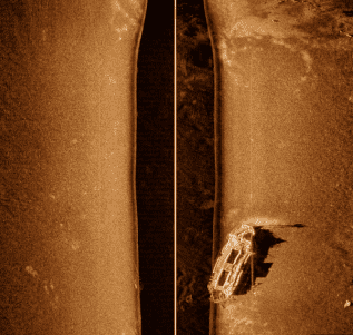
They distort correct image processing due to the similarity of their gray level to certain zones of foreground objects. Classical Otsu’s technique results in the segmented image with these artifacts as we can see below:

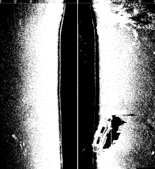
otsu_sss – LearnOpenCV — Pic 3 SSS sea bottom image

The method based on Otsu’s binarization was developed to deal with this spot challenge constraining the search range of the appropriate segmentation threshold for foreground object division. The improved Otsu’s method pipeline is the following:

Obtain Otsu’s threshold $T$
Apply Canny edge detection to compute $N_{30}$
if $N_{30} > 300$ compute final $T$ value.

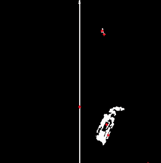
The result is clear wrecked ship separation from the background:

improved_otsu – LearnOpenCV — Pic 4 Improved Otsus result

Method Implementation

Let’s implement Otsu’s method on our own. It will look similar to threshold_otsu solution from the scikit-learn library, so feel free to use it as a reference. The function is built around maximization of the between-class variance (as we remember there is also minimization option) as OpenCV getThreshVal_Otsu.

The below image is used as input:

boat_initial – LearnOpenCV — Pic 5 Input image

Now let’s go through the following necessary points in order to achieve the result.

1. Read Image.
First, we need to read image in a grayscale mode and its possible improvement with a Gaussian blur in order to reduce the noise:

Download Code To easily follow along this tutorial, please download code by clicking on the button below. It's FREE!

Click here to download the source code to this post

C++

// Include Libraries
#include <iostream>
#include <opencv2/opencv.hpp>
#include <opencv2/imgproc.hpp>

using namespace std;
using namespace cv;

int main(){

 // read the image in BGR format
 Mat testImage = imread("boat.jpg", 0);

Python

# Read the image in a grayscale mode
image = cv2.imread(img_title, 0)

# Apply GaussianBlur to reduce image noise if it is required
if is_reduce_noise:
   image = cv2.GaussianBlur(image, (5, 5), 0)

In our case the image is quite qualitative, hence we set is_reduce_noise flag to False.

2. Calculate the Otsu’s threshold.
The below code block represents the main algorithm computation part concluding in the threshold obtaining. The precise explanations of the lines can be found in the comments:

C++

int bins_num = 256;

// Get the histogram
long double histogram[256];

// initialize all intensity values to 0
for(int i = 0; i < 256; i++)
    histogram[i] = 0;

// calculate the no of pixels for each intensity values
for(int y = 0; y < testImage.rows; y++)
    for(int x = 0; x < testImage.cols; x++)
        histogram[(int)testImage.at<uchar>(y,x)]++;

// Calculate the bin_edges
long double bin_edges[256];
bin_edges[0] = 0.0;
long double increment = 0.99609375;
for(int i = 1; i < 256; i++)
    bin_edges[i] = bin_edges[i-1] + increment;

// Calculate bin_mids
long double bin_mids[256];
for(int i = 0; i < 256; i++)
 bin_mids[i] = (bin_edges[i] + bin_edges[i+1])/2;

// Iterate over all thresholds (indices) and get the probabilities weight1, weight2
long double weight1[256];
weight1[0] = histogram[0];
for(int i = 1; i < 256; i++)
 weight1[i] = histogram[i] + weight1[i-1];

int total_sum=0;
for(int i = 0; i < 256; i++)
    total_sum = total_sum + histogram[i];
long double weight2[256];
weight2[0] = total_sum;
for(int i = 1; i < 256; i++)
 weight2[i] = weight2[i-1] - histogram[i - 1];

// Calculate the class means: mean1 and mean2
long double histogram_bin_mids[256];
for(int i = 0; i < 256; i++)
 histogram_bin_mids[i] = histogram[i] * bin_mids[i];

long double cumsum_mean1[256];
cumsum_mean1[0] = histogram_bin_mids[0];
for(int i = 1; i < 256; i++)
 cumsum_mean1[i] = cumsum_mean1[i-1] + histogram_bin_mids[i];

long double cumsum_mean2[256];
cumsum_mean2[0] = histogram_bin_mids[255];
for(int i = 1, j=254; i < 256 && j>=0; i++, j--)
 cumsum_mean2[i] = cumsum_mean2[i-1] + histogram_bin_mids[j];

long double mean1[256];
for(int i = 0; i < 256; i++)
 mean1[i] = cumsum_mean1[i] / weight1[i];

long double mean2[256];
for(int i = 0, j = 255; i < 256 && j >= 0; i++, j--)
 mean2[j] = cumsum_mean2[i] / weight2[j];

// Calculate Inter_class_variance
long double Inter_class_variance[255];
long double dnum = 10000000000;
for(int i = 0; i < 255; i++)
 Inter_class_variance[i] = ((weight1[i] * weight2[i] * (mean1[i] - mean2[i+1])) / dnum) * (mean1[i] - mean2[i+1]); 

// Maximize interclass variance
long double maxi = 0;
int getmax = 0;
for(int i = 0;i < 255; i++){
 if(maxi < Inter_class_variance[i]){
  maxi = Inter_class_variance[i];
  getmax = i;
 }
}

cout << "Otsu's algorithm implementation thresholding result: " << bin_mids[getmax];

Python

# Set total number of bins in the histogram
bins_num = 256

# Get the image histogram
hist, bin_edges = np.histogram(image, bins=bins_num)

# Get normalized histogram if it is required
if is_normalized:
    hist = np.divide(hist.ravel(), hist.max())

# Calculate centers of bins
bin_mids = (bin_edges[:-1] + bin_edges[1:]) / 2.

# Iterate over all thresholds (indices) and get the probabilities w1(t), w2(t)
weight1 = np.cumsum(hist)
weight2 = np.cumsum(hist[::-1])[::-1]

# Get the class means mu0(t)
mean1 = np.cumsum(hist * bin_mids) / weight1
# Get the class means mu1(t)
mean2 = (np.cumsum((hist * bin_mids)[::-1]) / weight2[::-1])[::-1]

inter_class_variance = weight1[:-1] * weight2[1:] * (mean1[:-1] - mean2[1:]) ** 2

# Maximize the inter_class_variance function val
index_of_max_val = np.argmax(inter_class_variance)

threshold = bin_mids[:-1][index_of_max_val]
print("Otsu's algorithm implementation thresholding result: ", threshold)

3. Results.
The execution result is:

Otsu's algorithm implementation thresholding result: 131.982421875

Now we better understand the algorithm’s essence after its whole pipeline implementation. Let’s explore how we can obtain the same result using the already implemented threshold method from the OpenCV library.

1. Read Image.
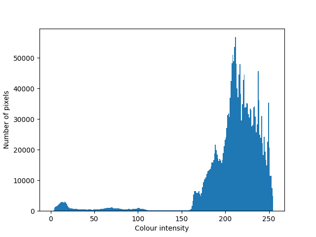
The first step is the same – image loading in a grayscale mode with a possible noise reduction. Let’s visualize the results of the preprocessed image and its histogram:

processed_img-1 – LearnOpenCV — Pic 6 Preprocessed image

In the below image histogram we can see clearly expressed mono peak and its near region and slightly expressed peak at the beginning of the scale:

image_hist – LearnOpenCV — Pic 7 Image histogram

2. Calculate the Otsu’s threshold.
To apply Otsu’s technique we simply need to use OpenCV threshold function with set THRESH_OTSU flag:

C++

Mat testImage = imread("boat.jpg", 0);

Mat dst;
double thresh = 0;
double maxValue = 255;

long double thres = cv::threshold(testImage,dst, thresh, maxValue, THRESH_OTSU);

cout << "Otsu Threshold : " << thres <<endl;

Python

# Applying Otsu's method setting the flag value into cv.THRESH_OTSU.
# Use a bimodal image as an input.
# Optimal threshold value is determined automatically.
otsu_threshold, image_result = cv2.threshold(
    image, 0, 255, cv2.THRESH_BINARY + cv2.THRESH_OTSU,
)
print("Obtained threshold: ", otsu_threshold)

3. Results.
The threshold value is near the obtained above in a handmade case (131.98):

Obtained threshold:  132.0

Now let’s view the final binarized image after Otsu’s method application:

otsu_result – LearnOpenCV — Pic 8 Otsus method result

We can clearly observe that the background and the main objects in the picture were separated. Let’s draw a histogram for the obtained binarized image:

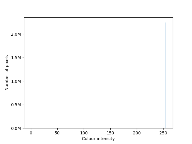
image_hist_res – LearnOpenCV — Pic 9 Otsus method result

As we can see, image pixels are now separated into 2 clusters with intensities values 0 and 255.

Otsu’s Thresholding with OpenCV

What is Image Thresholding?

Image Tresholding vs. Image Segmentation

Otsu’s Thresholding Concept

Otsu’s Binarization Application

Method Implementation

C++

Python

C++

Python

C++

Python

Get Started with OpenCV

Subscribe to receive the download link, receive updates, and be notified of bug fixes

Which email should I send you the download link?