Optical Flow in OpenCV (C++/Python)

In this post, we will learn about the various algorithms for calculating Optical Flow in a video or sequence of frames. We will discuss the relevant theory and implementation in OpenCV of sparse and dense optical flow algorithms. We share code in C++ and Python. Specifically, you will learn the following:

1. What is Optical Flow
   • Theory
   • Applications
2. Types: Sparse and Dense Optical Flow
3. Sparse Optical Flow using Lukas Kanade
   • Algorithm
   • Implementation in OpenCV
4. Dense Optical Flow in OpenCV
   • Dense Pyramid Lucas Kanade algorithm
   • Farneback Algorithm
   • RLOF algorithm
5. Summary

What is Optical Flow?

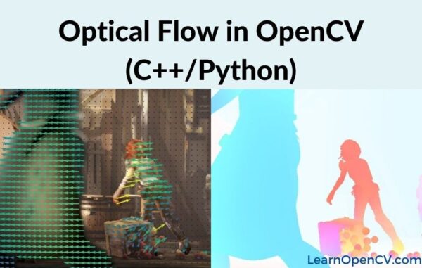
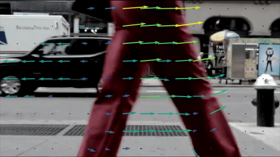
Optical flow is a task of per-pixel motion estimation between two consecutive frames in one video. Basically, the Optical Flow task implies the calculation of the shift vector for pixel as an object displacement difference between two neighboring images. The main idea of Optical Flow is to estimate the object’s displacement vector caused by it’s motion or camera movements.

Theoretical basics

Let’s assume that we have a gray-scale image – the matrix with pixel intensity. We define the function , where – pixel coordinates and – frame number. The function defines the exact pixel intensity at the frame .

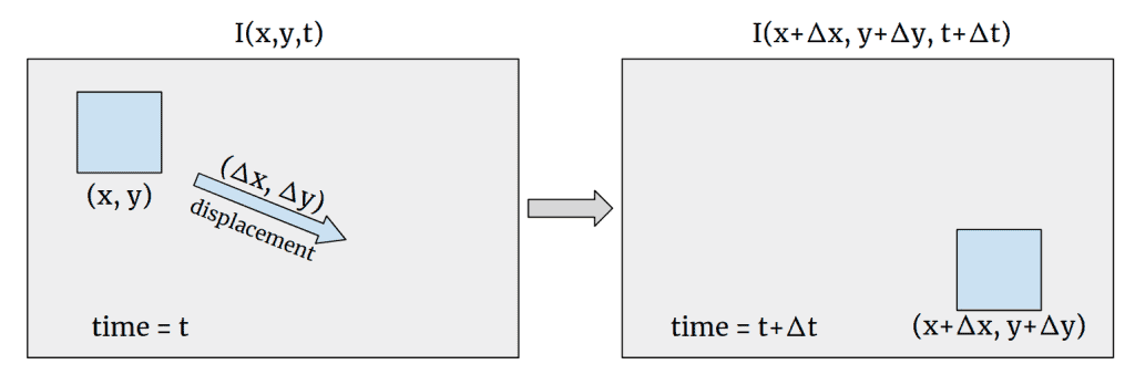
To start with, we assume that the object displacement doesn’t change the pixels intensity that belongs to the exact object, it means that . In our case . The major concern is to find the motion vector . Let’s take a look at graphical representation:

Using Taylor series expansion we can rewrite as , where and are image gradients. It is important that here we assume that parts of higher-order Taylor series are negligible, so this is a function approximation using only first-order Taylor’s expansion. The pixel motion difference between two frames and can be written as . Now, we have two variables and only one equation, so we can’t solve the equation right now, but we can use some tricks which will be disclosed in the following algorithms.

Optical Flow applications

Optical Flow can be used in many areas where the object’s motion information is crucial. Optical Flow is commonly found in video editors for compression, stabilization, slow-motion, etc. Also, Optical Flow finds its application in Action Recognition tasks and real-time tracking systems.

Sparse and Dense Optical Flow

There are two types of Optical Flow, and the first one is called Sparse Optical Flow. It computes the motion vector for the specific set of objects (for example – detected corners on image). Hence, it requires some preprocessing to extract features from the image, which will be the basement for the Optical Flow calculation. OpenCV provides some algorithm implementations to solve the Sparse Optical Flow task:

• Pyramid Lucas-Kanade
• Sparse RLOF

Using only a sparse feature set means that we will not have the motion information about pixels that are not contained in it. This restriction can be lifted using Dense Optical Flow algorithms which are supposed to calculate a motion vector for every pixel in the image. Some Dense Optical Flow algorithms are already implemented in OpenCV:

• Dense Pyramid Lucas-Kanade
• Farneback
• PCAFlow
• SimpleFlow
• RLOF
• DeepFlow
• DualTVL1

In this post we will take a look at the theoretical aspects of some of these algorithms and their usage with OpenCV.

Sparse Optical Flow

Lucas-Kanade algorithm

The Lucas-Kanade method is commonly used to calculate the Optical Flow for a sparse feature set. The main idea of this method based on a local motion constancy assumption, where nearby pixels have the same displacement direction. This assumption helps to get the approximated solution for the equation with two variables.

Theory

Let’s assume that the neighboring pixels have the same motion vector . We can take a fixed-size window to create a system of equations. Let be the pixel coordinates in the chosen window of elements . Hence, we can define the equation system as:

This equation system can be rewritten in matrix form:

As a result, we have a matrix equation: . Using the Least Squares we can compute the answer vector :

Lucas-Kanade algorithm improvements

The Optical Flow algorithms really suffer from abrupt movements due to the algorithm’s limitations. The common approach in practice is to use a multi-scaling trick. We need to create a so-called image pyramid, where every next image will be bigger than the previous one by some scaling factor (for example scale factor is 2). In terms of the fixed-size window, the abrupt movement on the small-sized image is more noticeable rather than on the large one. The founded displacement vectors in the small images will be used on the next larger pyramid stages to achieve better results.

As we mentioned before, Dense Optical Flow algorithms calculate the motion vector for the sparse feature set, so the common approach here is to use the Shi-Tomasi corner detector. It is used to find corners in the image and then calculate the corners’ motion vector between two consecutive frames.

Lucas-Kanade implementation with OpenCV

OpenCV has the implementation of Pyramid Lucas & Kanade with Shi-Tomasi algorithm improvement to calculate the Optical Flow. Let’s take a look at the OpenCV algorithm based on official documentation.

At first, we need to read our video and get the Shi-Tomasi algorithm’s features from the first frame. Also, some preprocessing things for algorithms and visualization are required here.

Python:

def lucas_kanade_method(video_path):
    # Read the video 
    cap = cv2.VideoCapture(video_path)

    # Parameters for ShiTomasi corner detection
    feature_params = dict(maxCorners=100, qualityLevel=0.3, minDistance=7, blockSize=7)

    # Parameters for Lucas Kanade optical flow
    lk_params = dict(
        winSize=(15, 15),
        maxLevel=2,
        criteria=(cv2.TERM_CRITERIA_EPS | cv2.TERM_CRITERIA_COUNT, 10, 0.03),
    )

    # Create random colors
    color = np.random.randint(0, 255, (100, 3))

    # Take first frame and find corners in it
    ret, old_frame = cap.read()
    old_gray = cv2.cvtColor(old_frame, cv2.COLOR_BGR2GRAY)
    p0 = cv2.goodFeaturesToTrack(old_gray, mask=None, **feature_params)

    # Create a mask image for drawing purposes
    mask = np.zeros_like(old_frame)

C++:

int lucas_kanade(const string& filename)
{
    // Read the video 
    VideoCapture capture(filename);
    if (!capture.isOpened()){
        //error in opening the video input
        cerr << "Unable to open file!" << endl;
        return 0;
    }

    // Create random colors
    vector<Scalar> colors;
    RNG rng;
    for(int i = 0; i < 100; i++)
    {
        int r = rng.uniform(0, 256);
        int g = rng.uniform(0, 256);
        int b = rng.uniform(0, 256);
        colors.push_back(Scalar(r,g,b));
    }

    Mat old_frame, old_gray;
    vector<Point2f> p0, p1;

    // Read first frame and find corners in it
    capture >> old_frame;
    cvtColor(old_frame, old_gray, COLOR_BGR2GRAY);
    goodFeaturesToTrack(old_gray, p0, 100, 0.3, 7, Mat(), 7, false, 0.04);

    // Create a mask image for drawing purposes
    Mat mask = Mat::zeros(old_frame.size(), old_frame.type());

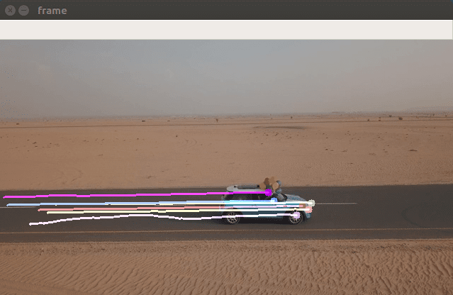
After that, we can start our demo. This is a cycled process, where we read a new video frame and calculate Shi-Tomasi features and Optical Flow in a loop. The calculated Optical Flow is shown as colored curves.

Python:

while True:
    # Read new frame
    ret, frame = cap.read()
    if not ret:
        break
    frame_gray = cv2.cvtColor(frame, cv2.COLOR_BGR2GRAY)

    # Calculate Optical Flow
    p1, st, err = cv2.calcOpticalFlowPyrLK(
        old_gray, frame_gray, p0, None, **lk_params
    )
    # Select good points
    good_new = p1[st == 1]
    good_old = p0[st == 1]

    # Draw the tracks
    for i, (new, old) in enumerate(zip(good_new, good_old)):
        a, b = new.ravel()
        c, d = old.ravel()
        mask = cv2.line(mask, (a, b), (c, d), color[i].tolist(), 2)
        frame = cv2.circle(frame, (a, b), 5, color[i].tolist(), -1)

    # Display the demo
    img = cv2.add(frame, mask)
    cv2.imshow("frame", img)
    k = cv2.waitKey(25) & 0xFF
    if k == 27:
        break

    # Update the previous frame and previous points
    old_gray = frame_gray.copy()
    p0 = good_new.reshape(-1, 1, 2)

C++:

while(true){
    // Read new frame
    Mat frame, frame_gray;
    capture >> frame;
    if (frame.empty())
        break;
    cvtColor(frame, frame_gray, COLOR_BGR2GRAY);

    // Calculate optical flow
    vector<uchar> status;
    vector<float> err;
    TermCriteria criteria = TermCriteria((TermCriteria::COUNT) + (TermCriteria::EPS), 10, 0.03);
    calcOpticalFlowPyrLK(old_gray, frame_gray, p0, p1, status, err, Size(15,15), 2, criteria);
    vector<Point2f> good_new;

    // Visualization part
    for(uint i = 0; i < p0.size(); i++)
    {
        // Select good points
        if(status[i] == 1) {
            good_new.push_back(p1[i]);
            // Draw the tracks
            line(mask,p1[i], p0[i], colors[i], 2);
            circle(frame, p1[i], 5, colors[i], -1);
        }
    }

    // Display the demo
    Mat img;
    add(frame, mask, img);
    if (save) {
        string save_path = "./optical_flow_frames/frame_" + to_string(counter) + ".jpg";
        imwrite(save_path, img);
    }
    imshow("flow", img);
    int keyboard = waitKey(25);
    if (keyboard == 'q' || keyboard == 27)
        break;

    // Update the previous frame and previous points
    old_gray = frame_gray.clone();
    p0 = good_new;
    counter++;
}

In short, this script takes two consecutive frames and finds the corners on the first one with cv2.goodFeaturesToTrack function. After that, we compute the Optical Flow with the Lucas-Kanade algorithm using the information about the corner location. This is a cycled process which does the same for each pair of consecutive images.

To run the Lucas-Kanade demo you can use the following command:

Python:

python3 demo.py --algorithm lucaskanade --video_path videos/car.mp4

C++:

./OpticalFlow ../videos/car.mp4 lucaskanade

As a result, you will see the demo video with pixel displacement curves:

To quit from the demo you can press the Esc button.

Dense Optical Flow

In this section, we will take a look at some Dense Optical Flow algorithms which can calculate the motion vector for every pixel in the image.

Implementation

Since the OpenCV Dense Optical Flow algorithms have the same usage pattern, we’ve created the wrapper function for convenience and code duplication avoiding.

At first, we need to read the first video frame and do image preprocessing if necessary:

Python:

def dense_optical_flow(method, video_path, params=[], to_gray=False):
    # Read the video and first frame
    cap = cv2.VideoCapture(video_path)
    ret, old_frame = cap.read()

    # crate HSV & make Value a constant
    hsv = np.zeros_like(old_frame)
    hsv[..., 1] = 255

    # Preprocessing for exact method
    if to_gray:
        old_frame = cv2.cvtColor(old_frame, cv2.COLOR_BGR2GRAY)

C++:

template <typename Method, typename... Args>
void dense_optical_flow(string filename, Method method, bool to_gray, Args&&... args)
{
    // Read the video and first frame
    VideoCapture capture(samples::findFile(filename));
    if (!capture.isOpened()) {
        //error in opening the video input
        cerr << "Unable to open file!" << endl;
    }
    Mat frame1, prvs;
    capture >> frame1;
    
    # Preprocessing for exact method
    if (to_gray)
        cvtColor(frame1, prvs, COLOR_BGR2GRAY);
    else
        prvs = frame1;

The main part of the demo is a loop, where we calculate Optical Flow for each new pair of consecutive images. After that, we encode the result into HSV format for visualization purposes:

Python:

while True:
    # Read the next frame
    ret, new_frame = cap.read()
    frame_copy = new_frame
    if not ret:
        break

    # Preprocessing for exact method
    if to_gray:
        new_frame = cv2.cvtColor(new_frame, cv2.COLOR_BGR2GRAY)

    # Calculate Optical Flow
    flow = method(old_frame, new_frame, None, *params)

    # Encoding: convert the algorithm's output into Polar coordinates
    mag, ang = cv2.cartToPolar(flow[..., 0], flow[..., 1])
    # Use Hue and Value to encode the Optical Flow
    hsv[..., 0] = ang * 180 / np.pi / 2
    hsv[..., 2] = cv2.normalize(mag, None, 0, 255, cv2.NORM_MINMAX)

    # Convert HSV image into BGR for demo
    bgr = cv2.cvtColor(hsv, cv2.COLOR_HSV2BGR)
    cv2.imshow("frame", frame_copy)
    cv2.imshow("optical flow", bgr)
    k = cv2.waitKey(25) & 0xFF
    if k == 27:
        break

    # Update the previous frame
    old_frame = new_frame

C++:

while (true) {
    // Read the next frame
    Mat frame2, next;
    capture >> frame2;
    if (frame2.empty())
        break;

    // Preprocessing for exact method
    if (to_gray)
        cvtColor(frame2, next, COLOR_BGR2GRAY);
    else
        next = frame2;

    // Calculate Optical Flow
    Mat flow(prvs.size(), CV_32FC2);
    method(prvs, next, flow, std::forward<Args>(args)...);

    // Visualization part
    Mat flow_parts[2];
    split(flow, flow_parts);

    // Convert the algorithm's output into Polar coordinates
    Mat magnitude, angle, magn_norm;
    cartToPolar(flow_parts[0], flow_parts[1], magnitude, angle, true);
    normalize(magnitude, magn_norm, 0.0f, 1.0f, NORM_MINMAX);
    angle *= ((1.f / 360.f) * (180.f / 255.f));

    // Build hsv image
    Mat _hsv[3], hsv, hsv8, bgr;
    _hsv[0] = angle;
    _hsv[1] = Mat::ones(angle.size(), CV_32F);
    _hsv[2] = magn_norm;
    merge(_hsv, 3, hsv);
    hsv.convertTo(hsv8, CV_8U, 255.0);
    
    // Display the results
    cvtColor(hsv8, bgr, COLOR_HSV2BGR);
    if (save) {
        string save_path = "./optical_flow_frames/frame_" + to_string(counter) + ".jpg";
        imwrite(save_path, bgr);
    }
    imshow("frame", frame2);
    imshow("flow", bgr);
    int keyboard = waitKey(30);
    if (keyboard == 'q' || keyboard == 27)
        break;

    // Update the previous frame
    prvs = next;
    counter++;
}

Therefore, this function reads two consecutive frames as method input. In some cases, the image grayscaling is needed, so the to_gray parameter should be set as True. After we got the algorithm output, we encode it for proper visualization using HSV color format.

Algorithm visualization

The dense optical flow algorithm output can be encoded as the HSV color scheme. Using the cv2.cartToPolar function, we can convert the displacement coordinates into polar coordinates as magnitude and angle for every pixel. Here we can encode angle and magnitude as Hue and Value respectively, while Saturation remains constant. To show the optical flow properly, we need to convert the HSV into BGR format.

Dense Pyramid Lucas-Kanade algorithm

To carry on with a Lucas-Kanade, OpenCV allows using this method not only for Sparse tasks but also for Dense Optical Flow calculation. The main technique here is to use Sparse algorithm output and make the interpolation on the whole image to get the motion vector for every pixel.

Dense Pyramid Lucas-Kanade with OpenCV

Let’s get back to the Dense Lucas-Kanade method. It is already implemented as calcOpticalFlowSparseToDense function. In the main function we should mention the method to use in our wrapper:

Python:

elif args.algorithm == 'lucaskanade_dense':
    method = cv2.optflow.calcOpticalFlowSparseToDense
    frames = dense_optical_flow(method, video_path, save, to_gray=True)

C++:

else if (method == "lucaskanade_dense"){
    dense_optical_flow(filename, optflow::calcOpticalFlowSparseToDense, to_gray, 8, 128, 0.05f, true, 500.0f, 1.5f); // default OpenCV params
}

This method requires the 1-D image as input, so we convert our BGR image to a gray-scale with cv2.cvtColor:

Python:

if to_gray:
    new_frame = cv2.cvtColor(new_frame, cv2.COLOR_BGR2GRAY)

C++:

if (to_gray)
    cvtColor(frame1, prvs, COLOR_BGR2GRAY);

You can run the algorithm demo using this command:

Python:

python3 demo.py --algorithm lucaskanade_dense --video_path videos/people.mp4

C++:

./OpticalFlow ../videos/car.mp4 lucaskanade_dense

It will start the demo, where each pixel displacement is encoded as HSV color:

Farneback algorithm

Let’s go further with the algorithms, and our next step is a Farneback algorithm. It was introduced in 2003, and it is used to calculate the optical flow for each pixel in the image.

Theory

The main idea of this method is to approximate some neighbors of each pixel with a polynomial: . Generally speaking, in the Lucas-Canade method we used the linear approximation since we had only first-order Taylor’s expansion. Now, we are increasing the accuracy of approximation with second-order values. Here, the idea leads to observing the differences in the approximated polynomials caused by object displacements. Our goal here is to calculate a displacement in the equation using the polynomial approximation.

The additional information about the algorithm and it’s improvements you can find in the original paper.

Farneback implementation with OpenCV

The OpenCV Farneback algorithm requires a 1-dimensional input image, so we convert the BRG image into gray-scale. In the main function we now can call our dense_optical_flow wrapper to start the Farneback’s demo with cv2.calcOpticalFlowFarneback function:

Python:

elif args.algorithm == 'farneback':
    method = cv2.calcOpticalFlowFarneback
    params = [0.5, 3, 15, 3, 5, 1.2, 0]  # default Farneback's algorithm parameters
    frames = dense_optical_flow(method, video_path, save, params, to_gray=True)

C++:

else if (method == "farneback"){
    dense_optical_flow(filename, calcOpticalFlowFarneback, to_gray, 0.5, 
    3, 15, 3, 5, 1.2, 0); // default OpenCV params
}

To run the Farneback demo, you can use the following script:

Python:

python3 demo.py --algorithm farneback --video_path videos/people.mp4

C++:

./OpticalFlow ../videos/car.mp4 farneback

RLOF

The Robust Local Optical Flow algorithm was published in 2016. The main idea of this work is that the intensity constancy assumption doesn’t fully reflect how the real world behaves. There are also shadows, reflections, weather conditions, moving light sources, and, in short, varying illuminations.

Theory

The RLOF algorithm is based on an illumination model proposed by Gennert and Negahdaripour in 1995: , where are the illumination model parameters. Like in the previous algorithms, there is a local motion constancy assumption supplemented with illumination constancy. Mathematically, it means that the vector is constant for every local image region.

The authors define the minimization function based on the illumination model and optimization method that works iteratively until the convergence. The optimization process is described in the original paper.

RLOF implementation with OpenCV

RLOF algorithm, in contrast to Farneback, requires the 3-channel image, so there is no preprocessing here. Now our method has changed to cv2.optflow.calcOpticalFlowDenseRLOF:

Python:

elif args.algorithm == "rlof":
    method = cv2.optflow.calcOpticalFlowDenseRLOF
    frames = dense_optical_flow(method, video_path, save)

C++:

else if (method == "rlof"){
    to_gray = false;
    dense_optical_flow(
       filename, optflow::calcOpticalFlowDenseRLOF, to_gray, 
       Ptr<cv::optflow::RLOFOpticalFlowParameter>(), 1.f, Size(6,6), 
       cv::optflow::InterpolationType::INTERP_EPIC, 128, 0.05f, 999.0f,
       15, 100, true, 500.0f, 1.5f, false); // default OpenCV params
}

To run the RLOF demo you can use the following script:

Python:

python3 demo.py --algorithm rlof --video_path videos/people.mp4

C++:

./OpticalFlow ../videos/car.mp4 rlof

Summary

In this post we considered the Optical Flow task which is indispensable when we need information about object motion. We took a look at some classical algorithms, their theoretical ideas, and practical usage with OpenCV library. Actually, the Optical Flow estimation is not limited to the algorithmic approach. The new approaches based on Deep Learning have led to quality improvement of Optical Flow estimation and this topic will be revealed in the next blog post.

Subscribe & Download Code

If you liked this article and would like to download code (C++ and Python) and example images used in this post, please subscribe to our newsletter. You will also receive a free Computer Vision Resource Guide. In our newsletter, we share OpenCV tutorials and examples written in C++/Python, and Computer Vision and Machine Learning algorithms and news.