Object Detection With Depth Measurement Using Pre-trained Models With OAK-D

This is the third blog post in the Oak series. If you haven’t checked out the previous posts on OAK, check them below.

• Introduction to OAK-D and DepthAI
• Stereo Vision and Depth Estimation using OpenCV AI Kit

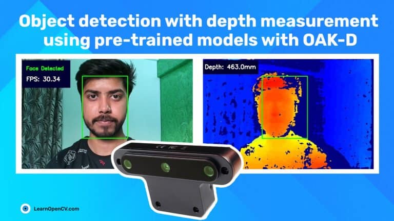
In this post, we are going to look at how we can run an existing pre-trained model on the oak device and get an inference from it.

1. A brief overview/recap of OAK and DepthAI
2. Supported models
3. Sources of pre-trained models
4. Available Neural Network nodes overview
5. Pipeline Overview
6. Code: Running a pre-trained face detection model
7. Output
8. Conclusion

1. A Brief Overview of OAK-D and DepthAI

In the previous posts, we got an overview of OAK-D and saw how it offers different cameras to calculate disparity and depth.

OAK-D and Oak-D Lite are not just stereo cameras but also equipped with a Myriad X VPU onboard. VPU, aka Visual Processing Unit, allows OAK-D to perform multiple operations onboard the device like Image manipulations (warping, dewarping, resizing, crop, edge detection, etc.), RGB depth alignment, tracking, and you can even run custom computer vision functions.

The VPU supports the inference of neural networks (as long as it is converted to the blob format). You can even run multiple AI models simultaneously, either in parallel or in series.

This ability of OAK makes it an all-in-one platform for your computer vision needs.

2. Supported Models

OAK cameras can run any AI model, even custom-architectured/built ones. It can even run multiple AI models at the same time, either in parallel or in series.

Before using your custom-trained models, you need to convert them into a MyriadX blob file format – so that they are optimized for the best inference on the MyriadX VPU processor.

Two conversion steps have to be taken to obtain a blob file:

• Use Model Optimizer to produce OpenVINO IR representation (where IR stands for Intermediate Representation)

• Use Model Compiler to convert IR representation into MyriadX blob

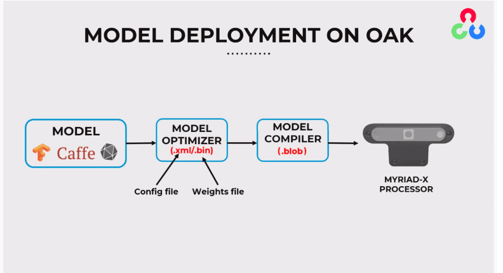
Higher-level solutions are also there to make you not get stuck on the model conversion process. You can visit the online MyriadX Blob converter that allows specifying different OpenVINO target versions and supports conversions from Tensorflow, Caffe, OpenVINO IR, and OpenVINO Model Zoo.

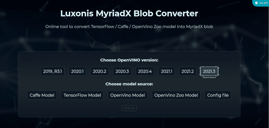
For automated usage of blob converter tool, there is a blobconverter PyPi package, that allows compiling MyriadX blobs both from the command line and from the Python script directly.

The latter is what we will be using in the below example.

3. Sources of Pre-trained Models

Following are the few sources that provide ready-to-deploy trained models for OAK.

Open Model Zoo

Open Model Zoo provides a wide variety of free, highly optimized, pre-trained deep-learning models that run blazingly fast on Intel CPUs, GPUs, and VPUs. 

This repository contains over 200 neural network models for tasks including Object Detection, Classification, Image Segmentation, Handwriting Recognition, Text-to-Speech, Human Pose Estimation, and others.

There are two kinds of models.

1. Intel’s Pre-Trained Models: The team at Intel has trained these models and optimized them to run with OpenVINO.

2. Public Pre-Trained Models: These are models created by the AI community and can be easily converted to OpenVINO format using OpenVINO Model Optimizer.

Luxonis Model Zoo

The OpenAi Kit is quickly becoming the go-to embedding platform of choice for many developers of computer vision applications. To aid the users in getting to know the platform’s capabilities better, Luxonis, the creators of OAK, have created DepthAI Model Zoo. It is a growing collection of ready-to-use open-source models for the Luxonis OpenCV AI Kit platform.

You can find models for tasks such as Monocular Depth Estimation, Object Detection, Segmentation, Facial Landmark Detection, Text Detection, Classification, and many more as new models are added to the model zoo.

Modelplace.ai

Modelplace.AI is a marketplace for machine learning models and a platform for the community to share their custom-trained models. 

It has a growing collection of OAK-compatible models for various Computer Vision tasks, be it Classification, Object Detection, Pose Estimation, or Text Detection.

It comes with a web interface to try out the model of your liking with your custom images. You can also compare models that perform similar tasks against one another on standard benchmarks.

Don’t forget to check out the previous post for Top sources to find Computer Vision Models.

4. Available Neural Network Nodes Overview

NeuralNetwork

This node runs neural inference using the defined model on input data. 

This node gives the raw output of the neural network, which means you have to decode the output yourself. 

This is the node you want to use when you are implementing your custom models.

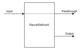
Input: 

1. Image to perform inference on

Outputs:

1. Raw neural network output
2. Input passthrough

Syntax:

pipeline = dai.Pipeline()
nn = pipeline.create(dai.node.NeuralNetwork)

MobileNetDetectionNetwork

MobileNet detection network node extends the NeuralNetwork node. 

The only difference is that this node is specifically for the MobileNet NN, and it decodes the result of the NN on the device. This means that out of this node is not a byte array but a ImgDetections that can easily be used in your code.

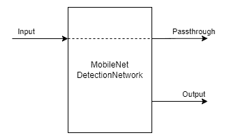
Inputs:

1. Image to perform detection on

Outputs:

1. Detection output
2. Input image passthrough

Syntax:

pipeline = dai.Pipeline()
mobilenetDet = pipeline.create(dai.node.MobileNetDetectionNetwork)

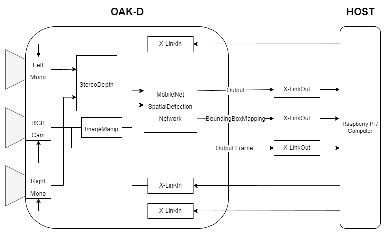
MobileNetSpatialDetectionNetwork

MobileNetSpatial detection network node works similarly to MobileNet, a detection network node, but along with the detection results, it also outputs the spatial location of the bounding box.

This network node mirrors the functionality of the spacial locator node on top of the mobilenet detection network node. SpacialLocator Node gives the average distance in the ROI of the depth frame.

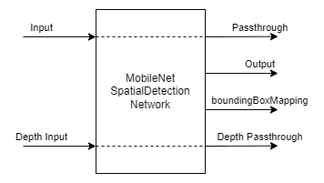
Inputs:

1. Image to perform detection on
2. Depth frame

Outputs:

1. Detection output
2. Input image passthrough
3. Depth passthrough

Syntax:

pipeline = dai.Pipeline()
mobilenetSpatial = pipeline.create(dai.node.MobileNetSpatialDetectionNetwork)

Similar to MobileNetDetectionNetwork and MobileNetSpatialDetectionNetwork, we have YoloDetectionNetwork and YoloSpatialDetectionNetwork to get the decoded detection and spatial detection output from a yolo network.

5. Pipeline

6. Code

Click here to download the source code to this post

Import Libraries

import cv2
import depthai as dai
import timeimport blobconverter

Define Frame size

FRAME_SIZE = (640, 360)

Define the NN model name and input size

Define the Input size, name, and the zoo name from where to download that model (only ‘DepthAI’ and ‘intel’ are supported at the time).

Note: If you define the path to the blob file directly, make sure the MODEL_NAME and ZOO_TYPE are None

For this demo, we use the “face-detection-retail-0004” face detection model from DepthAI model zoo.

DET_INPUT_SIZE = (300, 300)
model_name = "face-detection-retail-0004"
zoo_type = "depthai"
blob_path = None

Create Pipeline

Start defining a pipeline

pipeline = dai.Pipeline()

Define a source – RGB camera

Get the RGB camera frame

cam = pipeline.createColorCamera()
cam.setPreviewSize(FRAME_SIZE[0], FRAME_SIZE[1])
cam.setInterleaved(False)
cam.setResolution(dai.ColorCameraProperties.SensorResolution.THE_1080_P)
cam.setBoardSocket(dai.CameraBoardSocket.RGB)

Define mono camera sources for stereo depth

mono_left = pipeline.createMonoCamera()
mono_left.setResolution(dai.MonoCameraProperties.SensorResolution.THE_400_P)
mono_left.setBoardSocket(dai.CameraBoardSocket.LEFT)
mono_right = pipeline.createMonoCamera()
mono_right.setResolution(dai.MonoCameraProperties.SensorResolution.THE_400_P)
mono_right.setBoardSocket(dai.CameraBoardSocket.RIGHT)

Create stereo node

stereo = pipeline.createStereoDepth()

Linking mono cam outputs to stereo node

mono_left.out.link(stereo.left)
mono_right.out.link(stereo.right)

Use blobconverter to get the blob of the required model

We use the blobconverter to compile and download the model defined earlier from the selected model zoo, ‘depthai’ or ‘intel’.

We also specify the ‘shaves’ parameter. This tells the blobconverter to compile the model to run on the specified number of ‘shaves’.

The ‘shaves’ argument in blobconverter determines the number of SHAVE cores used to compile the neural network. The higher the value, the faster network can run.

if model_name is not None:
    blob_path = blobconverter.from_zoo(
        name=model_name,
        shaves=6,
        zoo_type=zoo_type
    )  

What are SHAVES?

The SHAVES are vector processors in DepthAI/OAK.  

Other than running the neural network, these SHAVES are also used for other things in the device, like handling the reformatting of images, doing some ISP, etc.

So, there is a limit to how many SHAVES you can use at once. The higher the resolution, the more SHAVES are consumed.

• For 1080p, 13 SHAVES (of 16) are free for neural network stuff.
• For 4K sensor resolution, 10 SHAVES are available for neural operations.

Define face detection NN node

face_spac_det_nn = pipeline.createMobileNetSpatialDetectionNetwork()
face_spac_det_nn.setConfidenceThreshold(0.75)
face_spac_det_nn.setBlobPath(blob_path)
face_spac_det_nn.setDepthLowerThreshold(100)
face_spac_det_nn.setDepthUpperThreshold(5000)

Define face detection input config

Preprocess the image frame for the Neural Network input. For that, we use the ImageManip node. 

ImageManip is the node that can apply different transformations on the input image and give the transformed image as the output. 

Here, this node is used to resize the image frame coming from the camera to the dimensions that our model accepts. We will learn more in-depth about this and other nodes in a later post on Creating a Complex Pipeline using DepthAI.

face_det_manip = pipeline.createImageManip()
face_det_manip.initialConfig.setResize(DET_INPUT_SIZE[0], DET_INPUT_SIZE[1])
face_det_manip.initialConfig.setKeepAspectRatio(False)

Linking

We link the RGB camera output to the ImageManip Node, the output of the ImageManip node to the Neural Network input, and the stereo depth output to the NN node.

cam.preview.link(face_det_manip.inputImage)
face_det_manip.out.link(face_spac_det_nn.input)stereo.depth.link(face_spac_det_nn.inputDepth)

Create preview output

Create a stream to get the output from the camera

x_preview_out = pipeline.createXLinkOut()
x_preview_out.setStreamName("preview")
cam.preview.link(x_preview_out.input)

Create detection output

Create a stream to get the output from the Neural Network

det_out = pipeline.createXLinkOut()
det_out.setStreamName('det_out')
face_spac_det_nn.out.link(det_out.input)

Define display function

We define a function to display info on the image frame

def display_info(frame, bbox, coordinates, status, status_color, fps):
    # Display bounding box
    cv2.rectangle(frame, bbox, status_color[status], 2)

    # Display coordinates
    if coordinates is not None:
        coord_x, coord_y, coord_z = coordinates
        cv2.putText(frame, f"X: {int(coord_x)} mm", (bbox[0] + 10, bbox[1] + 20), cv2.FONT_HERSHEY_TRIPLEX, 0.5, 255)
        cv2.putText(frame, f"Y: {int(coord_y)} mm", (bbox[0] + 10, bbox[1] + 35), cv2.FONT_HERSHEY_TRIPLEX, 0.5, 255)
        cv2.putText(frame, f"Z: {int(coord_z)} mm", (bbox[0] + 10, bbox[1] + 50), cv2.FONT_HERSHEY_TRIPLEX, 0.5, 255)

    # Create background for showing details
    cv2.rectangle(frame, (5, 5, 175, 100), (50, 0, 0), -1)

    # Display authentication status on the frame
    cv2.putText(frame, status, (20, 40), cv2.FONT_HERSHEY_SIMPLEX, 0.5, status_color[status])

    # Display instructions on the frame
    cv2.putText(frame, f'FPS: {fps:.2f}', (20, 80), cv2.FONT_HERSHEY_SIMPLEX, 0.6, (255, 255, 255))

Define some variables that we will use in the main loop

# Frame count
frame_count = 0

# Placeholder fps value
fps = 0

# Used to record the time when we processed last frames
prev_frame_time = 0

# Used to record the time at which we processed current frames
new_frame_time = 0

# Set status colors
status_color = {
    'Face Detected': (0, 255, 0),
    'No Face Detected': (0, 0, 255)
}

Main Loop

We start the pipeline and acquire video frames from the “preview” queue and get the NN outputs (detections and bounding box mapping) from the “det_out” queue.

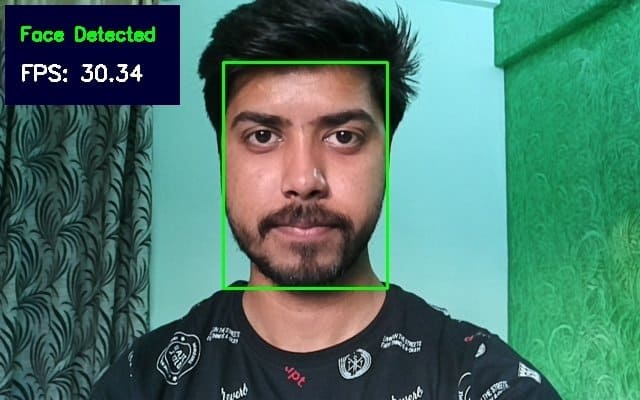
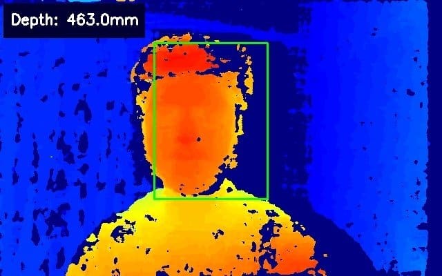
Once we have the outputs, we display the spacial information and bounding box on the image frame.

# Start pipeline
with dai.Device(pipeline) as device:

    # Output queue will be used to get the right camera frames from the outputs defined above
    q_cam = device.getOutputQueue(name="preview", maxSize=1, blocking=False)

    # Output queue will be used to get nn data from the video frames.
    q_det = device.getOutputQueue(name="det_out", maxSize=1, blocking=False)

    # # Output queue will be used to get nn data from the video frames.
    # q_bbox_depth_mapping = device.getOutputQueue(name="bbox_depth_mapping_out", maxSize=4, blocking=False)

    while True:
        # Get right camera frame
        in_cam = q_cam.get()
        frame = in_cam.getCvFrame()

        bbox = None
        coordinates = None

        inDet = q_det.tryGet()

        if inDet is not None:
            detections = inDet.detections

            # if face detected
            if len(detections) is not 0:
                detection = detections[0]

                # Correct bounding box
                xmin = max(0, detection.xmin)
                ymin = max(0, detection.ymin)
                xmax = min(detection.xmax, 1)
                ymax = min(detection.ymax, 1)

                # Calculate coordinates
                x = int(xmin*FRAME_SIZE[0])
                y = int(ymin*FRAME_SIZE[1])
                w = int(xmax*FRAME_SIZE[0]-xmin*FRAME_SIZE[0])
                h = int(ymax*FRAME_SIZE[1]-ymin*FRAME_SIZE[1])

                bbox = (x, y, w, h)

                # Get spacial coordinates
                coord_x = detection.spatialCoordinates.x
                coord_y = detection.spatialCoordinates.y
                coord_z = detection.spatialCoordinates.z

                coordinates = (coord_x, coord_y, coord_z)

        # Check if a face was detected in the frame
        if bbox:
            # Face detected
            status = 'Face Detected'
        else:
            # No face detected
            status = 'No Face Detected'

        # Display info on frame
        display_info(frame, bbox, coordinates, status, status_color, fps)

        # Calculate average fps
        if frame_count % 10 == 0:
            # Time when we finish processing last 100 frames
            new_frame_time = time.time()

            # Fps will be number of frame processed in one second
            fps = 1 / ((new_frame_time - prev_frame_time)/10)
            prev_frame_time = new_frame_time

        # Capture the key pressed
        key_pressed = cv2.waitKey(1) & 0xff

        # Stop the program if Esc key was pressed
        if key_pressed == 27:
            break

        # Display the final frame
        cv2.imshow("Face Cam", frame)

        # Increment frame count
        frame_count += 1

cv2.destroyAllWindows()

7. Output

8. Conclusion

This is all about how you can incorporate any pre-trained model in our pipeline.

The next post of this series will explore the other Pipeline nodes available to us and how they can be used together to create complex pipelines.