Welcome to this comprehensive guide on object detection using the latest “KerasCV YOLOv8” model.
YOLO object detection models have found their way into countless applications, from surveillance systems to autonomous vehicles. But, what happens when you pair this capability of YOLOv8 under the KerasCV framework? Recently, KerasCV has integrated the famous YOLOv8 detection models into its library. In this article, we explore how to fine-tune YOLOv8 with a custom dataset. Along the way, we will also cover the following points.
- Fine-tuning YOLOv8 on a traffic light detection dataset.
- Running inference on the validation images.
- Analyzing the results.
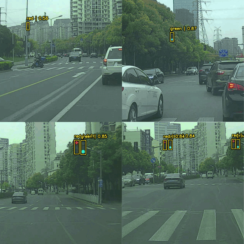
Table of Contents
YOLO Master Post – Every Model Explained
Don’t miss out on this comprehensive resource, Mastering All Yolo Models for a richer, more informed perspective on the YOLO series.
The Traffic Light Detection Dataset
We will train the KerasCV YOLOv8 model using a traffic light detection dataset. The Small Traffic Light Dataset (S2TLD) by Thinklab. The collection of the images and annotations are provided in the download link within the notebook.
The dataset contains 4564 images and the annotations are present in XML format. The following images paint a clear picture of the varying scenarios in which the images have been collected.
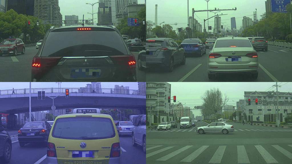
The dataset version that will be used contains four classes:
- red
- yellow
- green
- off
Object Detection using KerasCV YOLOv8
Let’s begin with the setup of the necessary libraries.
!pip install keras-cv==0.5.1
!pip install keras-core
In the initial step, the environment is set up to utilize the capabilities of “KerasCV YOLOv8” for object detection. Installing keras-cv and keras-core ensures the availability of all necessary modules to begin the object detection journey. It is important to maintain the right versions to prevent compatibility issues.In this tutorial, we’re using version 0.5.1 of keras-cv for the best results with YOLOv8.
Managing the Imports
The next step is importing the required packages and libraries.
import os
import xml.etree.ElementTree as ET
import tensorflow as tf
import keras_cv
import requests
import zipfile

from tqdm.auto import tqdm
from tensorflow import keras
from keras_cv import bounding_box
from keras_cv import visualization
Before diving into the core functionalities of “KerasCV YOLOv8” for object detection, let’s set the groundwork by importing the necessary libraries and modules:
os: Helps in interfacing with the underlying operating system that Python is running on. Useful for directory operations.
xml.etree.ElementTree (ET): Will assist in parsing XML files, commonly used in datasets with annotated object locations.
tensorflow & keras: The foundation upon which “KerasCV YOLOv8” is built, enabling deep learning capabilities.
keras_cv: A vital library that brings in the tools to leverage the YOLOv8 model for our project.
requests: This module lets us send HTTP requests, which might be essential for fetching online datasets or model weights.
zipfile: Handy for extracting compressed files, potentially useful if dealing with zipped datasets or model files.
tqdm: Enhances the code with progress bars, making lengthy processes user-friendly.
bounding_box & visualization from keras_cv: These are crucial for handling bounding box operations and visualizing results, respectively, after detecting objects using KerasCV YOLOv8.
By ensuring these modules are imported, we’re ready to proceed with the rest of the object detection process efficiently.
Downloading the Dataset
First, download the traffic light detection dataset from a direct source.
# Download dataset.
def download_file(url, save_name):
    if not os.path.exists(save_name):
        print(f"Downloading file")
        file = requests.get(url, stream=True)
        total_size = int(file.headers.get('content-length', 0))
        block_size = 1024
        progress_bar = tqdm(
            total=total_size,
            unit='iB',
            unit_scale=True
        )
        with open(os.path.join(save_name), 'wb') as f:
            for data in file.iter_content(block_size):
                progress_bar.update(len(data))
                f.write(data)
        progress_bar.close()
    else:
        print('File already present')

download_file(
    'https://www.dropbox.com/scl/fi/suext2oyjxa0v4p78bj3o/S2TLD_720x1280.zip?rlkey=iequuynn54uib0uhsc7eqfci4&dl=1',
    'S2TLD_720x1280.zip'
)
Unzip the dataset.
# Unzip the data file
def unzip(zip_file=None):
    try:
        with zipfile.ZipFile(zip_file) as z:
            z.extractall("./")
            print("Extracted all")
    except:
        print("Invalid file")

unzip('S2TLD_720x1280.zip')
The dataset will be extracted into the S2TLD_720x1280 directory.
Dataset and Training Parameters
The appropriate dataset and training parameters need to be defined. These include the dataset split for training and validation, the batch size, the learning rate, and the number of epochs the KerasCV YOLOv8 model needs to be trained for.
SPLIT_RATIO = 0.2
BATCH_SIZE = 8
LEARNING_RATE = 0.001
EPOCH = 75
GLOBAL_CLIPNORM = 10.0
20% of the data is reserved for validation, and the rest will be used for training. The batch size is 8 keeping in mind the model and image size to be used for training. The learning rate will be set at 0.001, and the model will be trained for 75 epochs.
The Dataset Preparation
Let’s move on to one of the most important aspects of training any deep learning model – preparing the dataset.
We start with defining the class names and accessing all the image and annotation files.
class_ids = [
    "red",
    "yellow",
    "green",
    "off",
]
class_mapping = dict(zip(range(len(class_ids)), class_ids))

# Path to images and annotations
path_images = "S2TLD_720x1280/images/"
path_annot = "S2TLD_720x1280/annotations/"

# Get all XML file paths in path_annot and sort them
xml_files = sorted(
    [
        os.path.join(path_annot, file_name)
        for file_name in os.listdir(path_annot)
        if file_name.endswith(".xml")
    ]
)

# Get all JPEG image file paths in path_images and sort them
jpg_files = sorted(
    [
        os.path.join(path_images, file_name)
        for file_name in os.listdir(path_images)
        if file_name.endswith(".jpg")
    ]
)
The class_mapping dictionary provides an easy lookup from numerical IDs to their respective class names. All the image and annotation file paths are stored in the xml_files and jpg_files , respectively.
Next is parsing the XML annotation files to store the labels and bounding box annotations needed for training.
def parse_annotation(xml_file):
    tree = ET.parse(xml_file)
    root = tree.getroot()

    image_name = root.find("filename").text
    image_path = os.path.join(path_images, image_name)

    boxes = []
    classes = []
    for obj in root.iter("object"):
        cls = obj.find("name").text
        classes.append(cls)

        bbox = obj.find("bndbox")
        xmin = float(bbox.find("xmin").text)
        ymin = float(bbox.find("ymin").text)
        xmax = float(bbox.find("xmax").text)
        ymax = float(bbox.find("ymax").text)
        boxes.append([xmin, ymin, xmax, ymax])

    class_ids = [
        list(class_mapping.keys())[list(class_mapping.values()).index(cls)]
        for cls in classes
    ]
    return image_path, boxes, class_ids


image_paths = []
bbox = []
classes = []
for xml_file in tqdm(xml_files):
    image_path, boxes, class_ids = parse_annotation(xml_file)
    image_paths.append(image_path)
    bbox.append(boxes)
    classes.append(class_ids)
The parse_annotation(xml_file) function dives into each XML file, extracting the filename, object classes, and their respective bounding box coordinates. With the help of class_mapping, it converts class names to class IDs for ease of use.
After parsing all XML files, we collect all image paths, bounding boxes, and class IDs in separate lists, which are then combined into a TensorFlow dataset using tf.data.Dataset.from_tensor_slices.
bbox = tf.ragged.constant(bbox)
classes = tf.ragged.constant(classes)
image_paths = tf.ragged.constant(image_paths)

data = tf.data.Dataset.from_tensor_slices((image_paths, classes, bbox))
All the data is not stored in a single tf.data.Dataset object. This needs to be divided between a training and validation set using SPLIT_RATIO.
# Determine the number of validation samples
num_val = int(len(xml_files) * SPLIT_RATIO)

# Split the dataset into train and validation sets
val_data = data.take(num_val)
train_data = data.skip(num_val)
Now, the task is to load the image and the annotations and also apply the required preprocessing.
def load_image(image_path):
    image = tf.io.read_file(image_path)
    image = tf.image.decode_jpeg(image, channels=3)
    return image

def load_dataset(image_path, classes, bbox):
    # Read Image
    image = load_image(image_path)
    bounding_boxes = {
        "classes": tf.cast(classes, dtype=tf.float32),
        "boxes": bbox,
    }
    return {"images": tf.cast(image, tf.float32), "bounding_boxes": bounding_boxes}

augmenter = keras.Sequential(
    layers=[
        keras_cv.layers.RandomFlip(mode="horizontal", bounding_box_format="xyxy"),
        keras_cv.layers.JitteredResize(
            target_size=(640, 640),
            scale_factor=(1.0, 1.0),
            bounding_box_format="xyxy",
        ),
    ]
)

train_ds = train_data.map(load_dataset, num_parallel_calls=tf.data.AUTOTUNE)
train_ds = train_ds.shuffle(BATCH_SIZE * 4)
train_ds = train_ds.ragged_batch(BATCH_SIZE, drop_remainder=True)
train_ds = train_ds.map(augmenter, num_parallel_calls=tf.data.AUTOTUNE)
For the training set, we resize the image to 640×640 resolution and apply the random horizontal flipping augmentation. The augmentation will ensure that the model does not overfit too early.
Coming to the validation set, this does not require any augmentation. Just resizing the images is enough.
resizing = keras_cv.layers.JitteredResize(
    target_size=(640, 640),
    scale_factor=(1.0, 1.0),
    bounding_box_format="xyxy",
)

val_ds = val_data.map(load_dataset, num_parallel_calls=tf.data.AUTOTUNE)
val_ds = val_ds.shuffle(BATCH_SIZE * 4)
val_ds = val_ds.ragged_batch(BATCH_SIZE, drop_remainder=True)
val_ds = val_ds.map(resizing, num_parallel_calls=tf.data.AUTOTUNE)
Before moving on to the next stage, let’s visualize a few samples using the training and validation dataset that was created above.
def visualize_dataset(inputs, value_range, rows, cols, bounding_box_format):
    inputs = next(iter(inputs.take(1)))
    images, bounding_boxes = inputs["images"], inputs["bounding_boxes"]
    visualization.plot_bounding_box_gallery(
        images,
        value_range=value_range,
        rows=rows,
        cols=cols,
        y_true=bounding_boxes,
        scale=5,
        font_scale=0.7,
        bounding_box_format=bounding_box_format,
        class_mapping=class_mapping,
    )


visualize_dataset(
    train_ds, bounding_box_format="xyxy", value_range=(0, 255), rows=2, cols=2
)

visualize_dataset(
    val_ds, bounding_box_format="xyxy", value_range=(0, 255), rows=2, cols=2
)
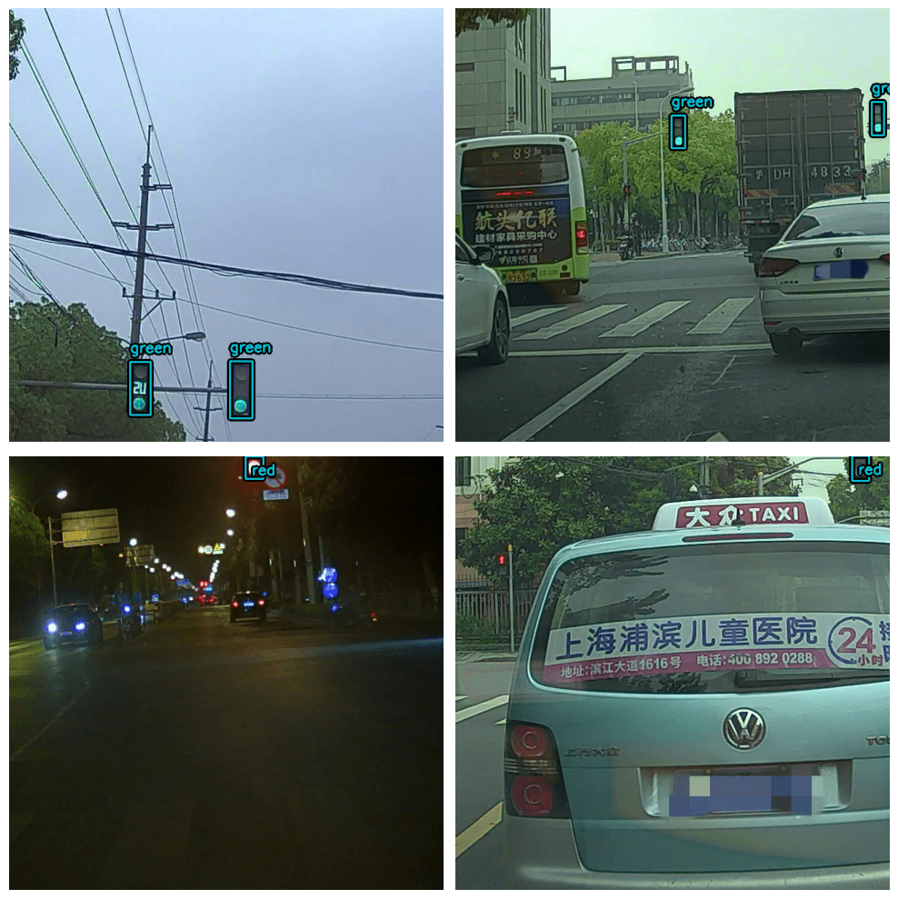
Here are a few outputs from the above visualization function.
Lastly, we need to create the final dataset format.
def dict_to_tuple(inputs):
    return inputs["images"], inputs["bounding_boxes"]


train_ds = train_ds.map(dict_to_tuple, num_parallel_calls=tf.data.AUTOTUNE)
train_ds = train_ds.prefetch(tf.data.AUTOTUNE)

val_ds = val_ds.map(dict_to_tuple, num_parallel_calls=tf.data.AUTOTUNE)
val_ds = val_ds.prefetch(tf.data.AUTOTUNE)
For the ease of model training, datasets are transformed using the dict_to_tuple function and optimized for better performance with prefetching.
The KerasCV YOLOv8 Model
We will create the KerasCV YOLOv8 model with a COCO pretrained backbone. The backbone is going to be YOLOv8 Large. From the entire pre-trained model, first load the backbone with the COCO pre-trained weights. Then, the entire YOLOv8 model will be created with randomly initialized weights for the head.
backbone = keras_cv.models.YOLOV8Backbone.from_preset(
    "yolo_v8_l_backbone_coco",
    load_weights=True
)

yolo = keras_cv.models.YOLOV8Detector(
    num_classes=len(class_mapping),
    bounding_box_format="xyxy",
    backbone=backbone,
    fpn_depth=3,
)

yolo.summary()
It is important to set the load_weights = True, else the COCO pretrained weights will not get loaded into the backbone
As our dataset annotation files are in XML format, all the bounding boxes are in XYXY format. So, the bounding_box_format is "xyxy" in the above code block. Furthermore, the fpn_depth is 3 as per the official KerasCV YOLOv8 documentation.
The next step is to define the optimizer and compile the model.
optimizer = tf.keras.optimizers.Adam(
    learning_rate=LEARNING_RATE,
    global_clipnorm=GLOBAL_CLIPNORM,
)

yolo.compile(
    optimizer=optimizer, classification_loss="binary_crossentropy", box_loss="ciou"
)
The learning rate is set as defined earlier, and the gradient clipping is incorporated using the global_clipnorm parameter. This ensures that gradients, which influence the model’s parameter updates, don’t become exceedingly large and destabilize training.
With the optimizer ready, we proceed to compile the YOLOv8 model. This prepares the model for training with the loss functions defined as follows:
classification_loss:"binary_crossentropy"is chosen as the classification loss.box_loss:"ciou"or Complete Intersection over Union is an advanced bounding box loss that accounts for both size and shape discrepancies between predicted and true boxes.
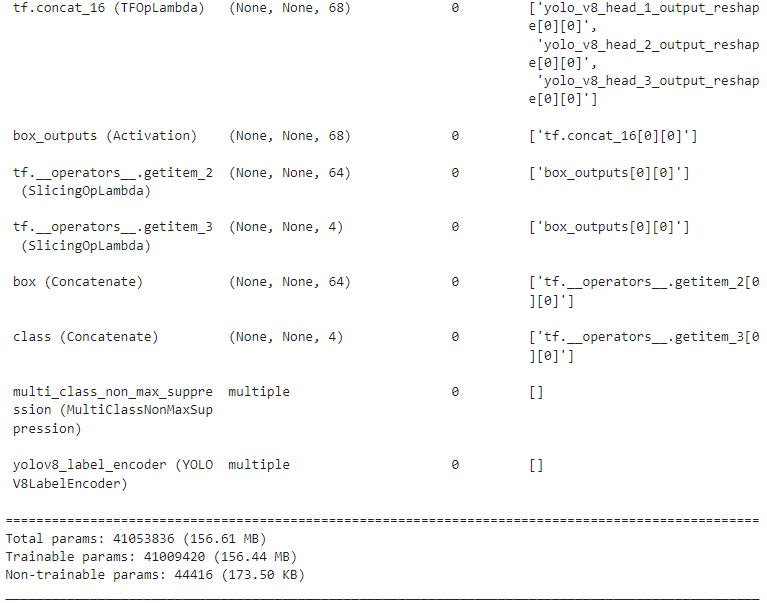
The final model that gets built contains 41 million parameters. Here is a snippet of the model summary, along with the number of trainable parameters.
The Evaluation Metrics
We choose the Mean Average Precision (mAP) as the evaluation metric. KerasCV already provides an optimized implementation of mAP for all of its object detection models.
class EvaluateCOCOMetricsCallback(keras.callbacks.Callback):
    def __init__(self, data, save_path):
        super().__init__()
        self.data = data
        self.metrics = keras_cv.metrics.BoxCOCOMetrics(
            bounding_box_format="xyxy",
            evaluate_freq=1e9,
        )

        self.save_path = save_path
        self.best_map = -1.0

    def on_epoch_end(self, epoch, logs):
        self.metrics.reset_state()
        for batch in self.data:
            images, y_true = batch[0], batch[1]
            y_pred = self.model.predict(images, verbose=0)
            self.metrics.update_state(y_true, y_pred)

        metrics = self.metrics.result(force=True)
        logs.update(metrics)

        current_map = metrics["MaP"]
        if current_map > self.best_map:
            self.best_map = current_map
            self.model.save(self.save_path)  # Save the model when mAP improves

        return logs
We define the EvaluateCOCOMetricsCallback with a custom Keras callback. This will be executed after every validation loop. If the current mAP is greater than the previous best mAP, then the model weights will be saved to disk.
Tensorboard Callback for Logging
Let’s also define a Tensorboard callback for the automatic logging of all the mAP and loss graphs.
tensorboard_callback = tf.keras.callbacks.TensorBoard(log_dir="logs_yolov8large")
All the Tensorboard logs will be stored in the logs_yolov8large directory.
Training the KerasCV YOLO8 Model on the Traffic Light Detection
We are now all set to start the training process. As all of our components are ready, we can simply call the yolo.fit() method to start the training.
history = yolo.fit(
    train_ds,
    validation_data=val_ds,
    epochs=EPOCH,
    callbacks=[
        EvaluateCOCOMetricsCallback(val_ds, "model_yolov8large.h5"),
        tensorboard_callback
    ],
)
The train_ds and val_ds are used as the training and validation datasets, respectively. Note that we also provide the callbacks that are defined in the previous section. The values of the mAP and loss will be stored in the history variable. However, it isn’t needed as everything is getting logged into Tensorboard.

The YOLOv8 model reaches the best mAP of more than 48%. This is where the best model weights are saved as well.
Inference on Validation Images
As we have the trained model with us now, it can be used to carry out inference on the images from the validation set.
def visualize_detections(model, dataset, bounding_box_format):
    for i in range(10):
        images, y_true = next(iter(dataset.take(i+1)))
        y_pred = model.predict(images)
        y_pred = bounding_box.to_ragged(y_pred)
        visualization.plot_bounding_box_gallery(
            images,
            value_range=(0, 255),
            bounding_box_format=bounding_box_format,
            # y_true=y_true,
            y_pred=y_pred,
            scale=4,
            rows=2,
            cols=2,
            show=True,
            font_scale=0.7,
            class_mapping=class_mapping,
        )
visualize_detections(yolo, dataset=val_ds, bounding_box_format="xyxy")
The above function loops over the data 10 times and carries out inference. After each inference, the results are plotted using the inbuilt plot_bounding_box_gallery function from KerasCV.
The following image shows some results where the predictions are correct.
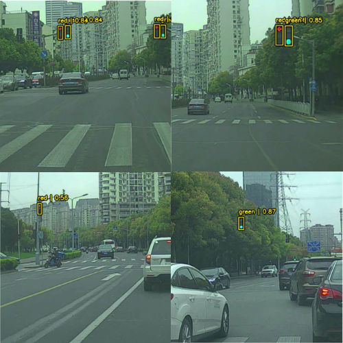
All the traffic light signs are predicted correctly by the model.
Even though the model achieved a very high accuracy, it’s not perfect yet. Here are some images where all the predicted results are not correct.
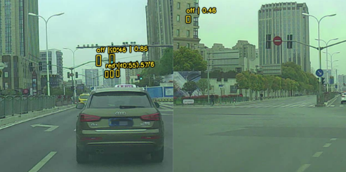
The above figure shows an image instance where the model predicts the window of the building as a traffic light. In another example, it is missing the predictions for a green and a red traffic light.
To mitigate the above situation, we can apply more augmentation to the images beyond horizontal flipping. KerasCV has a host of augmentations that can be used to reduce overfitting and improve accuracy in varying situations.
Video Inference using the Trained KerasCV YOLOv8 Model
We can also run video inference using the trained model. You can find the video inference scripts in the downloadable content and can run inference on your own videos. Here is an example command for running the video inference.
python infer_video.py --input inference_data/video.mov
The --input flag takes the path to a video file on which to run the inference. Following is a sample output of one such video inference experiment.
The results look good. The model is able to detect the traffic lights correctly in almost all the frames. There is a bit of flickering of course. But most probably, that will go away with a bit more training and augmentations.
Summary and Conclusion
This brings us to the end of this article. We started with the initial setup of KerasCV and moved on to the traffic light detection dataset. The preparation of the YOLOv8 detection model was also covered in detail, following which we carried out training and validation.
As KerasCV offers YOLOv8 as a core part of the library, there is potential for TensorFlow and Keras developers to build real-world applications. What project are you going to work on next? Let us know in the comments.




100K+ Learners
Join Free OpenCV Bootcamp3 Hours of Learning